NumPy - Quick Guide

NumPy is a Python package. It stands for 'Numerical Python'. It is a library consisting of multidimensional array objects and a collection of routines for processing of array.

Numeric, the ancestor of NumPy, was developed by Jim Hugunin. Another package Numarray was also developed, having some additional functionalities. In 2005, Travis Oliphant created NumPy package by incorporating the features of Numarray into Numeric package. There are many contributors to this open source project.

Operations using NumPy

Using NumPy, a developer can perform the following operations −

Mathematical and logical operations on arrays.
Fourier transforms and routines for shape manipulation.
Operations related to linear algebra. NumPy has in-built functions for linear algebra and random number generation.

NumPy – A Replacement for MatLab

NumPy is often used along with packages like SciPy (Scientific Python) and Mat−plotlib (plotting library). This combination is widely used as a replacement for MatLab, a popular platform for technical computing. However, Python alternative to MatLab is now seen as a more modern and complete programming language.

It is open source, which is an added advantage of NumPy.

NumPy - Environment

Standard Python distribution doesn't come bundled with NumPy module. A lightweight alternative is to install NumPy using popular Python package installer, pip.

pip install numpy

The best way to enable NumPy is to use an installable binary package specific to your operating system. These binaries contain full SciPy stack (inclusive of NumPy, SciPy, matplotlib, IPython, SymPy and nose packages along with core Python).

Windows

Anaconda (from https://www.continuum.io) is a free Python distribution for SciPy stack. It is also available for Linux and Mac.

Canopy (https://www.enthought.com/products/canopy/) is available as free as well as commercial distribution with full SciPy stack for Windows, Linux and Mac.

Python (x,y): It is a free Python distribution with SciPy stack and Spyder IDE for Windows OS. (Downloadable from https://www.python-xy.github.io/)

Linux

Package managers of respective Linux distributions are used to install one or more packages in SciPy stack.

For Ubuntu

sudo apt-get install python-numpy 
python-scipy python-matplotlibipythonipythonnotebook python-pandas 
python-sympy python-nose

For Fedora

sudo yum install numpyscipy python-matplotlibipython 
python-pandas sympy python-nose atlas-devel

Building from Source

Core Python (2.6.x, 2.7.x and 3.2.x onwards) must be installed with distutils and zlib module should be enabled.

GNU gcc (4.2 and above) C compiler must be available.

To install NumPy, run the following command.

Python setup.py install

To test whether NumPy module is properly installed, try to import it from Python prompt.

import numpy

If it is not installed, the following error message will be displayed.

Traceback (most recent call last): 
   File "<pyshell#0>", line 1, in <module> 
      import numpy 
ImportError: No module named 'numpy'

Alternatively, NumPy package is imported using the following syntax −

import numpy as np

NumPy - Ndarray Object

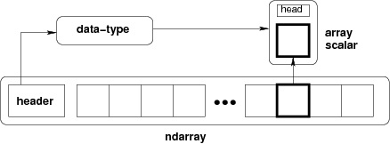
The most important object defined in NumPy is an N-dimensional array type called ndarray. It describes the collection of items of the same type. Items in the collection can be accessed using a zero-based index.

Every item in an ndarray takes the same size of block in the memory. Each element in ndarray is an object of data-type object (called dtype).

Any item extracted from ndarray object (by slicing) is represented by a Python object of one of array scalar types. The following diagram shows a relationship between ndarray, data type object (dtype) and array scalar type −

An instance of ndarray class can be constructed by different array creation routines described later in the tutorial. The basic ndarray is created using an array function in NumPy as follows −

numpy.array

It creates an ndarray from any object exposing array interface, or from any method that returns an array.

numpy.array(object, dtype = None, copy = True, order = None, subok = False, ndmin = 0)

The above constructor takes the following parameters −

Sr.No.	Parameter & Description
1	object Any object exposing the array interface method returns an array, or any (nested) sequence.
2	dtype Desired data type of array, optional
3	copy Optional. By default (true), the object is copied
4	order C (row major) or F (column major) or A (any) (default)
5	subok By default, returned array forced to be a base class array. If true, sub-classes passed through
6	ndmin Specifies minimum dimensions of resultant array

Take a look at the following examples to understand better.

Example 1

Live Demo

import numpy as np 
a = np.array([1,2,3]) 
print a

The output is as follows −

[1, 2, 3]

Example 2

Live Demo

# more than one dimensions 
import numpy as np 
a = np.array([[1, 2], [3, 4]]) 
print a

The output is as follows −

[[1, 2] 
 [3, 4]]

Example 3

Live Demo

# minimum dimensions 
import numpy as np 
a = np.array([1, 2, 3,4,5], ndmin = 2) 
print a

The output is as follows −

[[1, 2, 3, 4, 5]]

Example 4

Live Demo

# dtype parameter 
import numpy as np 
a = np.array([1, 2, 3], dtype = complex) 
print a

The output is as follows −

[ 1.+0.j,  2.+0.j,  3.+0.j]

The ndarray object consists of contiguous one-dimensional segment of computer memory, combined with an indexing scheme that maps each item to a location in the memory block. The memory block holds the elements in a row-major order (C style) or a column-major order (FORTRAN or MatLab style).

NumPy - Data Types

NumPy supports a much greater variety of numerical types than Python does. The following table shows different scalar data types defined in NumPy.

Sr.No.	Data Types & Description
1	bool_ Boolean (True or False) stored as a byte
2	int_ Default integer type (same as C long; normally either int64 or int32)
3	intc Identical to C int (normally int32 or int64)
4	intp Integer used for indexing (same as C ssize_t; normally either int32 or int64)
5	int8 Byte (-128 to 127)
6	int16 Integer (-32768 to 32767)
7	int32 Integer (-2147483648 to 2147483647)
8	int64 Integer (-9223372036854775808 to 9223372036854775807)
9	uint8 Unsigned integer (0 to 255)
10	uint16 Unsigned integer (0 to 65535)
11	uint32 Unsigned integer (0 to 4294967295)
12	uint64 Unsigned integer (0 to 18446744073709551615)
13	float_ Shorthand for float64
14	float16 Half precision float: sign bit, 5 bits exponent, 10 bits mantissa
15	float32 Single precision float: sign bit, 8 bits exponent, 23 bits mantissa
16	float64 Double precision float: sign bit, 11 bits exponent, 52 bits mantissa
17	complex_ Shorthand for complex128
18	complex64 Complex number, represented by two 32-bit floats (real and imaginary components)
19	complex128 Complex number, represented by two 64-bit floats (real and imaginary components)

NumPy numerical types are instances of dtype (data-type) objects, each having unique characteristics. The dtypes are available as np.bool_, np.float32, etc.

Data Type Objects (dtype)

A data type object describes interpretation of fixed block of memory corresponding to an array, depending on the following aspects −

Type of data (integer, float or Python object)
Size of data
Byte order (little-endian or big-endian)
In case of structured type, the names of fields, data type of each field and part of the memory block taken by each field.
If data type is a subarray, its shape and data type

The byte order is decided by prefixing '<' or '>' to data type. '<' means that encoding is little-endian (least significant is stored in smallest address). '>' means that encoding is big-endian (most significant byte is stored in smallest address).

A dtype object is constructed using the following syntax −

numpy.dtype(object, align, copy)

The parameters are −

Object − To be converted to data type object
Align − If true, adds padding to the field to make it similar to C-struct
Copy − Makes a new copy of dtype object. If false, the result is reference to builtin data type object

Example 1

Live Demo

# using array-scalar type 
import numpy as np 
dt = np.dtype(np.int32) 
print dt

The output is as follows −

int32

Example 2

Live Demo

#int8, int16, int32, int64 can be replaced by equivalent string 'i1', 'i2','i4', etc. 
import numpy as np 

dt = np.dtype('i4')
print dt

The output is as follows −

int32

Example 3

Live Demo

# using endian notation 
import numpy as np 
dt = np.dtype('>i4') 
print dt

The output is as follows −

>i4

The following examples show the use of structured data type. Here, the field name and the corresponding scalar data type is to be declared.

Example 4

Live Demo

# first create structured data type 
import numpy as np 
dt = np.dtype([('age',np.int8)]) 
print dt

The output is as follows −

[('age', 'i1')]

Example 5

Live Demo

# now apply it to ndarray object 
import numpy as np 

dt = np.dtype([('age',np.int8)]) 
a = np.array([(10,),(20,),(30,)], dtype = dt) 
print a

The output is as follows −

[(10,) (20,) (30,)]

Example 6

Live Demo

# file name can be used to access content of age column 
import numpy as np 

dt = np.dtype([('age',np.int8)]) 
a = np.array([(10,),(20,),(30,)], dtype = dt) 
print a['age']

The output is as follows −

[10 20 30]

Example 7

The following examples define a structured data type called student with a string field 'name', an integer field 'age' and a float field 'marks'. This dtype is applied to ndarray object.

Live Demo

import numpy as np 
student = np.dtype([('name','S20'), ('age', 'i1'), ('marks', 'f4')]) 
print student

The output is as follows −

[('name', 'S20'), ('age', 'i1'), ('marks', '<f4')])

Example 8

Live Demo

import numpy as np 

student = np.dtype([('name','S20'), ('age', 'i1'), ('marks', 'f4')]) 
a = np.array([('abc', 21, 50),('xyz', 18, 75)], dtype = student) 
print a

The output is as follows −

[('abc', 21, 50.0), ('xyz', 18, 75.0)]

Each built-in data type has a character code that uniquely identifies it.

'b' − boolean
'i' − (signed) integer
'u' − unsigned integer
'f' − floating-point
'c' − complex-floating point
'm' − timedelta
'M' − datetime
'O' − (Python) objects
'S', 'a' − (byte-)string
'U' − Unicode
'V' − raw data (void)

NumPy - Array Attributes

In this chapter, we will discuss the various array attributes of NumPy.

ndarray.shape

This array attribute returns a tuple consisting of array dimensions. It can also be used to resize the array.

Example 1

Live Demo

import numpy as np 
a = np.array([[1,2,3],[4,5,6]]) 
print a.shape

The output is as follows −

(2, 3)

Example 2

Live Demo

# this resizes the ndarray 
import numpy as np 

a = np.array([[1,2,3],[4,5,6]]) 
a.shape = (3,2) 
print a

The output is as follows −

[[1, 2] 
 [3, 4] 
 [5, 6]]

Example 3

NumPy also provides a reshape function to resize an array.

Live Demo

import numpy as np 
a = np.array([[1,2,3],[4,5,6]]) 
b = a.reshape(3,2) 
print b

The output is as follows −

[[1, 2] 
 [3, 4] 
 [5, 6]]

ndarray.ndim

This array attribute returns the number of array dimensions.

Example 1

Live Demo

# an array of evenly spaced numbers 
import numpy as np 
a = np.arange(24) 
print a

The output is as follows −

[0 1  2  3  4  5  6  7  8  9  10  11  12  13  14  15  16 17 18 19 20 21 22 23]

Example 2

Live Demo

# this is one dimensional array 
import numpy as np 
a = np.arange(24) 
a.ndim  

# now reshape it 
b = a.reshape(2,4,3) 
print b 
# b is having three dimensions

The output is as follows −

[[[ 0,  1,  2] 
  [ 3,  4,  5] 
  [ 6,  7,  8] 
  [ 9, 10, 11]]  
  [[12, 13, 14] 
   [15, 16, 17]
   [18, 19, 20] 
   [21, 22, 23]]]

numpy.itemsize

This array attribute returns the length of each element of array in bytes.

Example 1

Live Demo

# dtype of array is int8 (1 byte) 
import numpy as np 
x = np.array([1,2,3,4,5], dtype = np.int8) 
print x.itemsize

The output is as follows −

Example 2

Live Demo

# dtype of array is now float32 (4 bytes) 
import numpy as np 
x = np.array([1,2,3,4,5], dtype = np.float32) 
print x.itemsize

The output is as follows −

numpy.flags

The ndarray object has the following attributes. Its current values are returned by this function.

Sr.No.	Attribute & Description
1	C_CONTIGUOUS (C) The data is in a single, C-style contiguous segment
2	F_CONTIGUOUS (F) The data is in a single, Fortran-style contiguous segment
3	OWNDATA (O) The array owns the memory it uses or borrows it from another object
4	WRITEABLE (W) The data area can be written to. Setting this to False locks the data, making it read-only
5	ALIGNED (A) The data and all elements are aligned appropriately for the hardware
6	UPDATEIFCOPY (U) This array is a copy of some other array. When this array is deallocated, the base array will be updated with the contents of this array

Example

The following example shows the current values of flags.

Live Demo

import numpy as np 
x = np.array([1,2,3,4,5]) 
print x.flags

The output is as follows −

C_CONTIGUOUS : True 
F_CONTIGUOUS : True 
OWNDATA : True 
WRITEABLE : True 
ALIGNED : True 
UPDATEIFCOPY : False

NumPy - Array Creation Routines

A new ndarray object can be constructed by any of the following array creation routines or using a low-level ndarray constructor.

numpy.empty

It creates an uninitialized array of specified shape and dtype. It uses the following constructor −

numpy.empty(shape, dtype = float, order = 'C')

The constructor takes the following parameters.

Sr.No.	Parameter & Description
1	Shape Shape of an empty array in int or tuple of int
2	Dtype Desired output data type. Optional
3	Order 'C' for C-style row-major array, 'F' for FORTRAN style column-major array

Example

The following code shows an example of an empty array.

Live Demo

import numpy as np 
x = np.empty([3,2], dtype = int) 
print x

The output is as follows −

[[22649312    1701344351] 
 [1818321759  1885959276] 
 [16779776    156368896]]

Note − The elements in an array show random values as they are not initialized.

numpy.zeros

Returns a new array of specified size, filled with zeros.

numpy.zeros(shape, dtype = float, order = 'C')

The constructor takes the following parameters.

Sr.No.	Parameter & Description
1	Shape Shape of an empty array in int or sequence of int
2	Dtype Desired output data type. Optional
3	Order 'C' for C-style row-major array, 'F' for FORTRAN style column-major array

Example 1

Live Demo

# array of five zeros. Default dtype is float 
import numpy as np 
x = np.zeros(5) 
print x

The output is as follows −

[ 0.  0.  0.  0.  0.]

Example 2

Live Demo

import numpy as np 
x = np.zeros((5,), dtype = np.int) 
print x

Now, the output would be as follows −

[0  0  0  0  0]

Example 3

Live Demo

# custom type 
import numpy as np 
x = np.zeros((2,2), dtype = [('x', 'i4'), ('y', 'i4')])  
print x

It should produce the following output −

[[(0,0)(0,0)]
 [(0,0)(0,0)]]

numpy.ones

Returns a new array of specified size and type, filled with ones.

numpy.ones(shape, dtype = None, order = 'C')

The constructor takes the following parameters.

Sr.No.	Parameter & Description
1	Shape Shape of an empty array in int or tuple of int
2	Dtype Desired output data type. Optional
3	Order 'C' for C-style row-major array, 'F' for FORTRAN style column-major array

Example 1

Live Demo

# array of five ones. Default dtype is float 
import numpy as np 
x = np.ones(5) 
print x

The output is as follows −

[ 1.  1.  1.  1.  1.]

Example 2

Live Demo

import numpy as np 
x = np.ones([2,2], dtype = int) 
print x

Now, the output would be as follows −

[[1  1] 
 [1  1]]

NumPy - Array From Existing Data

In this chapter, we will discuss how to create an array from existing data.

numpy.asarray

This function is similar to numpy.array except for the fact that it has fewer parameters. This routine is useful for converting Python sequence into ndarray.

numpy.asarray(a, dtype = None, order = None)

The constructor takes the following parameters.

Sr.No.	Parameter & Description
1	a Input data in any form such as list, list of tuples, tuples, tuple of tuples or tuple of lists
2	dtype By default, the data type of input data is applied to the resultant ndarray
3	order C (row major) or F (column major). C is default

The following examples show how you can use the asarray function.

Example 1

Live Demo

# convert list to ndarray 
import numpy as np 

x = [1,2,3] 
a = np.asarray(x) 
print a

Its output would be as follows −

[1  2  3]

Example 2

Live Demo

# dtype is set 
import numpy as np 

x = [1,2,3]
a = np.asarray(x, dtype = float) 
print a

Now, the output would be as follows −

[ 1.  2.  3.]

Example 3

Live Demo

# ndarray from tuple 
import numpy as np 

x = (1,2,3) 
a = np.asarray(x) 
print a

Its output would be −

[1  2  3]

Example 4

Live Demo

# ndarray from list of tuples 
import numpy as np 

x = [(1,2,3),(4,5)] 
a = np.asarray(x) 
print a

Here, the output would be as follows −

[(1, 2, 3) (4, 5)]

numpy.frombuffer

This function interprets a buffer as one-dimensional array. Any object that exposes the buffer interface is used as parameter to return an ndarray.

numpy.frombuffer(buffer, dtype = float, count = -1, offset = 0)

The constructor takes the following parameters.

Sr.No.	Parameter & Description
1	buffer Any object that exposes buffer interface
2	dtype Data type of returned ndarray. Defaults to float
3	count The number of items to read, default -1 means all data
4	offset The starting position to read from. Default is 0

Example

The following examples demonstrate the use of frombuffer function.

Live Demo

import numpy as np 
s = 'Hello World' 
a = np.frombuffer(s, dtype = 'S1') 
print a

Here is its output −

['H'  'e'  'l'  'l'  'o'  ' '  'W'  'o'  'r'  'l'  'd']

numpy.fromiter

This function builds an ndarray object from any iterable object. A new one-dimensional array is returned by this function.

numpy.fromiter(iterable, dtype, count = -1)

Here, the constructor takes the following parameters.

Sr.No.	Parameter & Description
1	iterable Any iterable object
2	dtype Data type of resultant array
3	count The number of items to be read from iterator. Default is -1 which means all data to be read

The following examples show how to use the built-in range() function to return a list object. An iterator of this list is used to form an ndarray object.

Example 1

Live Demo

# create list object using range function 
import numpy as np 
list = range(5) 
print list

Its output is as follows −

[0,  1,  2,  3,  4]

Example 2

Live Demo

# obtain iterator object from list 
import numpy as np 
list = range(5) 
it = iter(list)  

# use iterator to create ndarray 
x = np.fromiter(it, dtype = float) 
print x

Now, the output would be as follows −

[0.   1.   2.   3.   4.]

NumPy - Array From Numerical Ranges

In this chapter, we will see how to create an array from numerical ranges.

numpy.arange

This function returns an ndarray object containing evenly spaced values within a given range. The format of the function is as follows −

numpy.arange(start, stop, step, dtype)

The constructor takes the following parameters.

Sr.No.	Parameter & Description
1	start The start of an interval. If omitted, defaults to 0
2	stop The end of an interval (not including this number)
3	step Spacing between values, default is 1
4	dtype Data type of resulting ndarray. If not given, data type of input is used

The following examples show how you can use this function.

Example 1

Live Demo

import numpy as np 
x = np.arange(5) 
print x

Its output would be as follows −

[0  1  2  3  4]

Example 2

Live Demo

import numpy as np 
# dtype set 
x = np.arange(5, dtype = float)
print x

Here, the output would be −

[0.  1.  2.  3.  4.]

Example 3

Live Demo

# start and stop parameters set 
import numpy as np 
x = np.arange(10,20,2) 
print x

Its output is as follows −

[10  12  14  16  18]

numpy.linspace

This function is similar to arange() function. In this function, instead of step size, the number of evenly spaced values between the interval is specified. The usage of this function is as follows −

numpy.linspace(start, stop, num, endpoint, retstep, dtype)

The constructor takes the following parameters.

Sr.No.	Parameter & Description
1	start The starting value of the sequence
2	stop The end value of the sequence, included in the sequence if endpoint set to true
3	num The number of evenly spaced samples to be generated. Default is 50
4	endpoint True by default, hence the stop value is included in the sequence. If false, it is not included
5	retstep If true, returns samples and step between the consecutive numbers
6	dtype Data type of output ndarray

The following examples demonstrate the use linspace function.

Example 1

Live Demo

import numpy as np 
x = np.linspace(10,20,5) 
print x

Its output would be −

[10.   12.5   15.   17.5  20.]

Example 2

Live Demo

# endpoint set to false 
import numpy as np 
x = np.linspace(10,20, 5, endpoint = False) 
print x

The output would be −

[10.   12.   14.   16.   18.]

Example 3

Live Demo

# find retstep value 
import numpy as np 

x = np.linspace(1,2,5, retstep = True) 
print x 
# retstep here is 0.25

Now, the output would be −

(array([ 1.  ,  1.25,  1.5 ,  1.75,  2.  ]), 0.25)

numpy.logspace

This function returns an ndarray object that contains the numbers that are evenly spaced on a log scale. Start and stop endpoints of the scale are indices of the base, usually 10.

numpy.logspace(start, stop, num, endpoint, base, dtype)

Following parameters determine the output of logspace function.

Sr.No.	Parameter & Description
1	start The starting point of the sequence is base^start
2	stop The final value of sequence is base^stop
3	num The number of values between the range. Default is 50
4	endpoint If true, stop is the last value in the range
5	base Base of log space, default is 10
6	dtype Data type of output array. If not given, it depends upon other input arguments

The following examples will help you understand the logspace function.

Example 1

Live Demo

import numpy as np 
# default base is 10 
a = np.logspace(1.0, 2.0, num = 10) 
print a

Its output would be as follows −

[ 10.           12.91549665     16.68100537      21.5443469  27.82559402      
  35.93813664   46.41588834     59.94842503      77.42636827    100.    ]

Example 2

Live Demo

# set base of log space to 2 
import numpy as np 
a = np.logspace(1,10,num = 10, base = 2) 
print a

Now, the output would be −

[ 2.     4.     8.    16.    32.    64.   128.   256.    512.   1024.]

NumPy - Indexing & Slicing

Contents of ndarray object can be accessed and modified by indexing or slicing, just like Python's in-built container objects.

As mentioned earlier, items in ndarray object follows zero-based index. Three types of indexing methods are available − field access, basic slicing and advanced indexing.

Basic slicing is an extension of Python's basic concept of slicing to n dimensions. A Python slice object is constructed by giving start, stop, and step parameters to the built-in slice function. This slice object is passed to the array to extract a part of array.

Example 1

Live Demo

import numpy as np 
a = np.arange(10) 
s = slice(2,7,2) 
print a[s]

Its output is as follows −

[2  4  6]

In the above example, an ndarray object is prepared by arange() function. Then a slice object is defined with start, stop, and step values 2, 7, and 2 respectively. When this slice object is passed to the ndarray, a part of it starting with index 2 up to 7 with a step of 2 is sliced.

The same result can also be obtained by giving the slicing parameters separated by a colon : (start:stop:step) directly to the ndarray object.

Example 2

Live Demo

import numpy as np 
a = np.arange(10) 
b = a[2:7:2] 
print b

Here, we will get the same output −

[2  4  6]

If only one parameter is put, a single item corresponding to the index will be returned. If a : is inserted in front of it, all items from that index onwards will be extracted. If two parameters (with : between them) is used, items between the two indexes (not including the stop index) with default step one are sliced.

Example 3

Live Demo

# slice single item 
import numpy as np 

a = np.arange(10) 
b = a[5] 
print b

Its output is as follows −

Example 4

Live Demo

# slice items starting from index 
import numpy as np 
a = np.arange(10) 
print a[2:]

Now, the output would be −

[2  3  4  5  6  7  8  9]

Example 5

Live Demo

# slice items between indexes 
import numpy as np 
a = np.arange(10) 
print a[2:5]

Here, the output would be −

[2  3  4]

The above description applies to multi-dimensional ndarray too.

Example 6

Live Demo

import numpy as np 
a = np.array([[1,2,3],[3,4,5],[4,5,6]]) 
print a  

# slice items starting from index
print 'Now we will slice the array from the index a[1:]' 
print a[1:]

The output is as follows −

[[1 2 3]
 [3 4 5]
 [4 5 6]]

Now we will slice the array from the index a[1:]
[[3 4 5]
 [4 5 6]]

Slicing can also include ellipsis (…) to make a selection tuple of the same length as the dimension of an array. If ellipsis is used at the row position, it will return an ndarray comprising of items in rows.

Example 7

Live Demo

# array to begin with 
import numpy as np 
a = np.array([[1,2,3],[3,4,5],[4,5,6]]) 

print 'Our array is:' 
print a 
print '\n'  

# this returns array of items in the second column 
print 'The items in the second column are:'  
print a[...,1] 
print '\n'  

# Now we will slice all items from the second row 
print 'The items in the second row are:' 
print a[1,...] 
print '\n'  

# Now we will slice all items from column 1 onwards 
print 'The items column 1 onwards are:' 
print a[...,1:]

The output of this program is as follows −

Our array is:
[[1 2 3]
 [3 4 5]
 [4 5 6]] 
 
The items in the second column are: 
[2 4 5] 

The items in the second row are:
[3 4 5]

The items column 1 onwards are:
[[2 3]
 [4 5]
 [5 6]]

NumPy - Advanced Indexing

It is possible to make a selection from ndarray that is a non-tuple sequence, ndarray object of integer or Boolean data type, or a tuple with at least one item being a sequence object. Advanced indexing always returns a copy of the data. As against this, the slicing only presents a view.

There are two types of advanced indexing − Integer and Boolean.

Integer Indexing

This mechanism helps in selecting any arbitrary item in an array based on its N-dimensional index. Each integer array represents the number of indexes into that dimension. When the index consists of as many integer arrays as the dimensions of the target ndarray, it becomes straightforward.

In the following example, one element of specified column from each row of ndarray object is selected. Hence, the row index contains all row numbers, and the column index specifies the element to be selected.

Example 1

Live Demo

import numpy as np 

x = np.array([[1, 2], [3, 4], [5, 6]]) 
y = x[[0,1,2], [0,1,0]] 
print y

Its output would be as follows −

[1  4  5]

The selection includes elements at (0,0), (1,1) and (2,0) from the first array.

In the following example, elements placed at corners of a 4X3 array are selected. The row indices of selection are [0, 0] and [3,3] whereas the column indices are [0,2] and [0,2].

Example 2

Live Demo

import numpy as np 
x = np.array([[ 0,  1,  2],[ 3,  4,  5],[ 6,  7,  8],[ 9, 10, 11]]) 
   
print 'Our array is:' 
print x 
print '\n' 

rows = np.array([[0,0],[3,3]])
cols = np.array([[0,2],[0,2]]) 
y = x[rows,cols] 
   
print 'The corner elements of this array are:' 
print y

The output of this program is as follows −

Our array is:                                                                 
[[ 0  1  2]                                                                   
 [ 3  4  5]                                                                   
 [ 6  7  8]                                                                   
 [ 9 10 11]]
 
The corner elements of this array are:                                        
[[ 0  2]                                                                      
 [ 9 11]]

The resultant selection is an ndarray object containing corner elements.

Advanced and basic indexing can be combined by using one slice (:) or ellipsis (…) with an index array. The following example uses slice for row and advanced index for column. The result is the same when slice is used for both. But advanced index results in copy and may have different memory layout.

Example 3

Live Demo

import numpy as np 
x = np.array([[ 0,  1,  2],[ 3,  4,  5],[ 6,  7,  8],[ 9, 10, 11]]) 

print 'Our array is:' 
print x 
print '\n'  

# slicing 
z = x[1:4,1:3] 

print 'After slicing, our array becomes:' 
print z 
print '\n'  

# using advanced index for column 
y = x[1:4,[1,2]] 

print 'Slicing using advanced index for column:' 
print y

The output of this program would be as follows −

Our array is:
[[ 0  1  2] 
 [ 3  4  5] 
 [ 6  7  8]
 [ 9 10 11]]
 
After slicing, our array becomes:
[[ 4  5]
 [ 7  8]
 [10 11]]

Slicing using advanced index for column:
[[ 4  5]
 [ 7  8]
 [10 11]]

Boolean Array Indexing

This type of advanced indexing is used when the resultant object is meant to be the result of Boolean operations, such as comparison operators.

Example 1

In this example, items greater than 5 are returned as a result of Boolean indexing.

Live Demo

import numpy as np 
x = np.array([[ 0,  1,  2],[ 3,  4,  5],[ 6,  7,  8],[ 9, 10, 11]]) 

print 'Our array is:' 
print x 
print '\n'  

# Now we will print the items greater than 5 
print 'The items greater than 5 are:' 
print x[x > 5]

The output of this program would be −

Our array is: 
[[ 0  1  2] 
 [ 3  4  5] 
 [ 6  7  8] 
 [ 9 10 11]] 
 
The items greater than 5 are:
[ 6  7  8  9 10 11]

Example 2

In this example, NaN (Not a Number) elements are omitted by using ~ (complement operator).

Live Demo

import numpy as np 
a = np.array([np.nan, 1,2,np.nan,3,4,5]) 
print a[~np.isnan(a)]

Its output would be −

[ 1.   2.   3.   4.   5.]

Example 3

The following example shows how to filter out the non-complex elements from an array.

Live Demo

import numpy as np 
a = np.array([1, 2+6j, 5, 3.5+5j]) 
print a[np.iscomplex(a)]

Here, the output is as follows −

[2.0+6.j  3.5+5.j]

NumPy - Broadcasting

The term broadcasting refers to the ability of NumPy to treat arrays of different shapes during arithmetic operations. Arithmetic operations on arrays are usually done on corresponding elements. If two arrays are of exactly the same shape, then these operations are smoothly performed.

Example 1

Live Demo

import numpy as np 

a = np.array([1,2,3,4]) 
b = np.array([10,20,30,40]) 
c = a * b 
print c

Its output is as follows −

[10   40   90   160]

If the dimensions of two arrays are dissimilar, element-to-element operations are not possible. However, operations on arrays of non-similar shapes is still possible in NumPy, because of the broadcasting capability. The smaller array is broadcast to the size of the larger array so that they have compatible shapes.

Broadcasting is possible if the following rules are satisfied −

Array with smaller ndim than the other is prepended with '1' in its shape.
Size in each dimension of the output shape is maximum of the input sizes in that dimension.
An input can be used in calculation, if its size in a particular dimension matches the output size or its value is exactly 1.
If an input has a dimension size of 1, the first data entry in that dimension is used for all calculations along that dimension.

A set of arrays is said to be broadcastable if the above rules produce a valid result and one of the following is true −

Arrays have exactly the same shape.
Arrays have the same number of dimensions and the length of each dimension is either a common length or 1.
Array having too few dimensions can have its shape prepended with a dimension of length 1, so that the above stated property is true.

The following program shows an example of broadcasting.

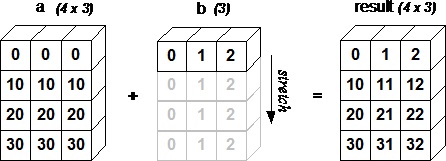
Example 2

Live Demo

import numpy as np 
a = np.array([[0.0,0.0,0.0],[10.0,10.0,10.0],[20.0,20.0,20.0],[30.0,30.0,30.0]]) 
b = np.array([1.0,2.0,3.0])  
   
print 'First array:' 
print a 
print '\n'  
   
print 'Second array:' 
print b 
print '\n'  
   
print 'First Array + Second Array' 
print a + b

The output of this program would be as follows −

First array:
[[ 0. 0. 0.]
 [ 10. 10. 10.]
 [ 20. 20. 20.]
 [ 30. 30. 30.]]

Second array:
[ 1. 2. 3.]

First Array + Second Array
[[ 1. 2. 3.]
 [ 11. 12. 13.]
 [ 21. 22. 23.]
 [ 31. 32. 33.]]

The following figure demonstrates how array b is broadcast to become compatible with a.

NumPy - Iterating Over Array

NumPy package contains an iterator object numpy.nditer. It is an efficient multidimensional iterator object using which it is possible to iterate over an array. Each element of an array is visited using Python’s standard Iterator interface.

Let us create a 3X4 array using arange() function and iterate over it using nditer.

Example 1

Live Demo

import numpy as np
a = np.arange(0,60,5)
a = a.reshape(3,4)

print 'Original array is:'
print a
print '\n'

print 'Modified array is:'
for x in np.nditer(a):
   print x,

The output of this program is as follows −

Original array is:
[[ 0 5 10 15]
 [20 25 30 35]
 [40 45 50 55]]

Modified array is:
0 5 10 15 20 25 30 35 40 45 50 55

Example 2

The order of iteration is chosen to match the memory layout of an array, without considering a particular ordering. This can be seen by iterating over the transpose of the above array.

Live Demo

import numpy as np 
a = np.arange(0,60,5) 
a = a.reshape(3,4) 
   
print 'Original array is:'
print a 
print '\n'  
   
print 'Transpose of the original array is:' 
b = a.T 
print b 
print '\n'  
   
print 'Modified array is:' 
for x in np.nditer(b): 
   print x,

The output of the above program is as follows −

Original array is:
[[ 0 5 10 15]
 [20 25 30 35]
 [40 45 50 55]]

Transpose of the original array is:
[[ 0 20 40]
 [ 5 25 45]
 [10 30 50]
 [15 35 55]]

Modified array is:
0 5 10 15 20 25 30 35 40 45 50 55

Iteration Order

If the same elements are stored using F-style order, the iterator chooses the more efficient way of iterating over an array.

Example 1

Live Demo

import numpy as np
a = np.arange(0,60,5)
a = a.reshape(3,4)
print 'Original array is:'
print a
print '\n'

print 'Transpose of the original array is:'
b = a.T
print b
print '\n'

print 'Sorted in C-style order:'
c = b.copy(order='C')
print c
for x in np.nditer(c):
   print x,

print '\n'

print 'Sorted in F-style order:'
c = b.copy(order='F')
print c
for x in np.nditer(c):
   print x,

Its output would be as follows −

Original array is:
[[ 0 5 10 15]
 [20 25 30 35]
 [40 45 50 55]]

Transpose of the original array is:
[[ 0 20 40]
 [ 5 25 45]
 [10 30 50]
 [15 35 55]]

Sorted in C-style order:
[[ 0 20 40]
 [ 5 25 45]
 [10 30 50]
 [15 35 55]]
0 20 40 5 25 45 10 30 50 15 35 55

Sorted in F-style order:
[[ 0 20 40]
 [ 5 25 45]
 [10 30 50]
 [15 35 55]]
0 5 10 15 20 25 30 35 40 45 50 55

Example 2

It is possible to force nditer object to use a specific order by explicitly mentioning it.

Live Demo

import numpy as np 
a = np.arange(0,60,5) 
a = a.reshape(3,4) 

print 'Original array is:' 
print a 
print '\n'  

print 'Sorted in C-style order:' 
for x in np.nditer(a, order = 'C'): 
   print x,  
print '\n' 

print 'Sorted in F-style order:' 
for x in np.nditer(a, order = 'F'): 
   print x,

Its output would be −

Original array is:
[[ 0 5 10 15]
 [20 25 30 35]
 [40 45 50 55]]

Sorted in C-style order:
0 5 10 15 20 25 30 35 40 45 50 55

Sorted in F-style order:
0 20 40 5 25 45 10 30 50 15 35 55

Modifying Array Values

The nditer object has another optional parameter called op_flags. Its default value is read-only, but can be set to read-write or write-only mode. This will enable modifying array elements using this iterator.

Example

Live Demo

import numpy as np
a = np.arange(0,60,5)
a = a.reshape(3,4)
print 'Original array is:'
print a
print '\n'

for x in np.nditer(a, op_flags = ['readwrite']):
   x[...] = 2*x
print 'Modified array is:'
print a

Its output is as follows −

Original array is:
[[ 0 5 10 15]
 [20 25 30 35]
 [40 45 50 55]]

Modified array is:
[[ 0 10 20 30]
 [ 40 50 60 70]
 [ 80 90 100 110]]

External Loop

The nditer class constructor has a ‘flags’ parameter, which can take the following values −

Sr.No.	Parameter & Description
1	c_index C_order index can be racked
2	f_index Fortran_order index is tracked
3	multi-index Type of indexes with one per iteration can be tracked
4	external_loop Causes values given to be one-dimensional arrays with multiple values instead of zero-dimensional array

Example

In the following example, one-dimensional arrays corresponding to each column is traversed by the iterator.

Live Demo

import numpy as np 
a = np.arange(0,60,5) 
a = a.reshape(3,4) 

print 'Original array is:' 
print a 
print '\n'  

print 'Modified array is:' 
for x in np.nditer(a, flags = ['external_loop'], order = 'F'): 
   print x,

The output is as follows −

Original array is:
[[ 0 5 10 15]
 [20 25 30 35]
 [40 45 50 55]]

Modified array is:
[ 0 20 40] [ 5 25 45] [10 30 50] [15 35 55]

Broadcasting Iteration

If two arrays are broadcastable, a combined nditer object is able to iterate upon them concurrently. Assuming that an array a has dimension 3X4, and there is another array b of dimension 1X4, the iterator of following type is used (array b is broadcast to size of a).

Example

Live Demo

import numpy as np 
a = np.arange(0,60,5) 
a = a.reshape(3,4) 

print 'First array is:' 
print a 
print '\n'  

print 'Second array is:' 
b = np.array([1, 2, 3, 4], dtype = int) 
print b  
print '\n' 

print 'Modified array is:' 
for x,y in np.nditer([a,b]): 
   print "%d:%d" % (x,y),

Its output would be as follows −

First array is:
[[ 0 5 10 15]
 [20 25 30 35]
 [40 45 50 55]]

Second array is:
[1 2 3 4]

Modified array is:
0:1 5:2 10:3 15:4 20:1 25:2 30:3 35:4 40:1 45:2 50:3 55:4

NumPy - Array Manipulation

Several routines are available in NumPy package for manipulation of elements in ndarray object. They can be classified into the following types −

Changing Shape

Sr.No.	Shape & Description
1	reshape Gives a new shape to an array without changing its data
2	flat A 1-D iterator over the array
3	flatten Returns a copy of the array collapsed into one dimension
4	ravel Returns a contiguous flattened array

Transpose Operations

Sr.No.	Operation & Description
1	transpose Permutes the dimensions of an array
2	ndarray.T Same as self.transpose()
3	rollaxis Rolls the specified axis backwards
4	swapaxes Interchanges the two axes of an array

Changing Dimensions

Sr.No.	Dimension & Description
1	broadcast Produces an object that mimics broadcasting
2	broadcast_to Broadcasts an array to a new shape
3	expand_dims Expands the shape of an array
4	squeeze Removes single-dimensional entries from the shape of an array

Joining Arrays

Sr.No.	Array & Description
1	concatenate Joins a sequence of arrays along an existing axis
2	stack Joins a sequence of arrays along a new axis
3	hstack Stacks arrays in sequence horizontally (column wise)
4	vstack Stacks arrays in sequence vertically (row wise)

Splitting Arrays

Sr.No.	Array & Description
1	split Splits an array into multiple sub-arrays
2	hsplit Splits an array into multiple sub-arrays horizontally (column-wise)
3	vsplit Splits an array into multiple sub-arrays vertically (row-wise)

Adding / Removing Elements

Sr.No.	Element & Description
1	resize Returns a new array with the specified shape
2	append Appends the values to the end of an array
3	insert Inserts the values along the given axis before the given indices
4	delete Returns a new array with sub-arrays along an axis deleted
5	unique Finds the unique elements of an array

NumPy - Binary Operators

Following are the functions for bitwise operations available in NumPy package.

Sr.No.	Operation & Description
1	bitwise_and Computes bitwise AND operation of array elements
2	bitwise_or Computes bitwise OR operation of array elements
3	invert Computes bitwise NOT
4	left_shift Shifts bits of a binary representation to the left
5	right_shift Shifts bits of binary representation to the right

NumPy - String Functions

The following functions are used to perform vectorized string operations for arrays of dtype numpy.string_ or numpy.unicode_. They are based on the standard string functions in Python's built-in library.

Sr.No.	Function & Description
1	add() Returns element-wise string concatenation for two arrays of str or Unicode
2	multiply() Returns the string with multiple concatenation, element-wise
3	center() Returns a copy of the given string with elements centered in a string of specified length
4	capitalize() Returns a copy of the string with only the first character capitalized
5	title() Returns the element-wise title cased version of the string or unicode
6	lower() Returns an array with the elements converted to lowercase
7	upper() Returns an array with the elements converted to uppercase
8	split() Returns a list of the words in the string, using separatordelimiter
9	splitlines() Returns a list of the lines in the element, breaking at the line boundaries
10	strip() Returns a copy with the leading and trailing characters removed
11	join() Returns a string which is the concatenation of the strings in the sequence
12	replace() Returns a copy of the string with all occurrences of substring replaced by the new string
13	decode() Calls str.decode element-wise
14	encode() Calls str.encode element-wise

These functions are defined in character array class (numpy.char). The older Numarray package contained chararray class. The above functions in numpy.char class are useful in performing vectorized string operations.

NumPy - Mathematical Functions

Quite understandably, NumPy contains a large number of various mathematical operations. NumPy provides standard trigonometric functions, functions for arithmetic operations, handling complex numbers, etc.

Trigonometric Functions

NumPy has standard trigonometric functions which return trigonometric ratios for a given angle in radians.

Example

Live Demo

import numpy as np 
a = np.array([0,30,45,60,90]) 

print 'Sine of different angles:' 
# Convert to radians by multiplying with pi/180 
print np.sin(a*np.pi/180) 
print '\n'  

print 'Cosine values for angles in array:' 
print np.cos(a*np.pi/180) 
print '\n'  

print 'Tangent values for given angles:' 
print np.tan(a*np.pi/180)

Here is its output −

Sine of different angles:                                                     
[ 0.          0.5         0.70710678  0.8660254   1.        ]

Cosine values for angles in array:
[  1.00000000e+00   8.66025404e-01   7.07106781e-01   5.00000000e-01
   6.12323400e-17]

Tangent values for given angles:                                              
[  0.00000000e+00   5.77350269e-01   1.00000000e+00   1.73205081e+00
   1.63312394e+16]

arcsin, arcos, and arctan functions return the trigonometric inverse of sin, cos, and tan of the given angle. The result of these functions can be verified by numpy.degrees() function by converting radians to degrees.

Example

Live Demo

import numpy as np 
a = np.array([0,30,45,60,90]) 

print 'Array containing sine values:' 
sin = np.sin(a*np.pi/180) 
print sin 
print '\n'  

print 'Compute sine inverse of angles. Returned values are in radians.' 
inv = np.arcsin(sin) 
print inv 
print '\n'  

print 'Check result by converting to degrees:' 
print np.degrees(inv) 
print '\n'  

print 'arccos and arctan functions behave similarly:' 
cos = np.cos(a*np.pi/180) 
print cos 
print '\n'  

print 'Inverse of cos:' 
inv = np.arccos(cos) 
print inv 
print '\n'  

print 'In degrees:' 
print np.degrees(inv) 
print '\n'  

print 'Tan function:' 
tan = np.tan(a*np.pi/180) 
print tan
print '\n'  

print 'Inverse of tan:' 
inv = np.arctan(tan) 
print inv 
print '\n'  

print 'In degrees:' 
print np.degrees(inv)

Its output is as follows −

Array containing sine values:
[ 0.          0.5         0.70710678  0.8660254   1.        ]

Compute sine inverse of angles. Returned values are in radians.
[ 0.          0.52359878  0.78539816  1.04719755  1.57079633] 

Check result by converting to degrees:
[  0.  30.  45.  60.  90.]

arccos and arctan functions behave similarly:
[  1.00000000e+00   8.66025404e-01   7.07106781e-01   5.00000000e-01          
   6.12323400e-17] 

Inverse of cos:
[ 0.          0.52359878  0.78539816  1.04719755  1.57079633] 

In degrees:
[  0.  30.  45.  60.  90.] 

Tan function:
[  0.00000000e+00   5.77350269e-01   1.00000000e+00   1.73205081e+00          
   1.63312394e+16]

Inverse of tan:
[ 0.          0.52359878  0.78539816  1.04719755  1.57079633]

In degrees:
[  0.  30.  45.  60.  90.]

Functions for Rounding

numpy.around()

This is a function that returns the value rounded to the desired precision. The function takes the following parameters.

numpy.around(a,decimals)

Where,

Sr.No.	Parameter & Description
1	a Input data
2	decimals The number of decimals to round to. Default is 0. If negative, the integer is rounded to position to the left of the decimal point

Example

Live Demo

import numpy as np 
a = np.array([1.0,5.55, 123, 0.567, 25.532]) 

print 'Original array:' 
print a 
print '\n'  

print 'After rounding:' 
print np.around(a) 
print np.around(a, decimals = 1) 
print np.around(a, decimals = -1)

It produces the following output −

Original array:                                                               
[   1.       5.55   123.       0.567   25.532] 

After rounding:                                                               
[   1.    6.   123.    1.   26. ]                                               
[   1.    5.6  123.    0.6  25.5]                                          
[   0.    10.  120.    0.   30. ]

numpy.floor()

This function returns the largest integer not greater than the input parameter. The floor of the scalar x is the largest integer i, such that i <= x. Note that in Python, flooring always is rounded away from 0.

Example

Live Demo

import numpy as np 
a = np.array([-1.7, 1.5, -0.2, 0.6, 10]) 

print 'The given array:' 
print a 
print '\n'  

print 'The modified array:' 
print np.floor(a)

It produces the following output −

The given array:                                                              
[ -1.7   1.5  -0.2   0.6  10. ]

The modified array:                                                           
[ -2.   1.  -1.   0.  10.]

numpy.ceil()

The ceil() function returns the ceiling of an input value, i.e. the ceil of the scalar x is the smallest integer i, such that i >= x.

Example

Live Demo

import numpy as np 
a = np.array([-1.7, 1.5, -0.2, 0.6, 10]) 

print 'The given array:' 
print a 
print '\n'  

print 'The modified array:' 
print np.ceil(a)

It will produce the following output −

The given array:                                                              
[ -1.7   1.5  -0.2   0.6  10. ]

The modified array:                                                           
[ -1.   2.  -0.   1.  10.]

NumPy - Arithmetic Operations

Input arrays for performing arithmetic operations such as add(), subtract(), multiply(), and divide() must be either of the same shape or should conform to array broadcasting rules.

Example

Live Demo

import numpy as np 
a = np.arange(9, dtype = np.float_).reshape(3,3) 

print 'First array:' 
print a 
print '\n'  

print 'Second array:' 
b = np.array([10,10,10]) 
print b 
print '\n'  

print 'Add the two arrays:' 
print np.add(a,b) 
print '\n'  

print 'Subtract the two arrays:' 
print np.subtract(a,b) 
print '\n'  

print 'Multiply the two arrays:' 
print np.multiply(a,b) 
print '\n'  

print 'Divide the two arrays:' 
print np.divide(a,b)

It will produce the following output −

First array:
[[ 0. 1. 2.]
 [ 3. 4. 5.]
 [ 6. 7. 8.]]

Second array:
[10 10 10]

Add the two arrays:
[[ 10. 11. 12.]
 [ 13. 14. 15.]
 [ 16. 17. 18.]]

Subtract the two arrays:
[[-10. -9. -8.]
 [ -7. -6. -5.]
 [ -4. -3. -2.]]

Multiply the two arrays:
[[ 0. 10. 20.]
 [ 30. 40. 50.]
 [ 60. 70. 80.]]

Divide the two arrays:
[[ 0. 0.1 0.2]
 [ 0.3 0.4 0.5]
 [ 0.6 0.7 0.8]]

Let us now discuss some of the other important arithmetic functions available in NumPy.

numpy.reciprocal()

This function returns the reciprocal of argument, element-wise. For elements with absolute values larger than 1, the result is always 0 because of the way in which Python handles integer division. For integer 0, an overflow warning is issued.

Example

Live Demo

import numpy as np 
a = np.array([0.25, 1.33, 1, 0, 100]) 

print 'Our array is:' 
print a 
print '\n'  

print 'After applying reciprocal function:' 
print np.reciprocal(a) 
print '\n'  

b = np.array([100], dtype = int) 
print 'The second array is:' 
print b 
print '\n'  

print 'After applying reciprocal function:' 
print np.reciprocal(b)

It will produce the following output −

Our array is:                                                                 
[   0.25    1.33    1.      0.    100.  ]

After applying reciprocal function:                                           
main.py:9: RuntimeWarning: divide by zero encountered in reciprocal
  print np.reciprocal(a)
[ 4.         0.7518797  1.               inf  0.01     ]

The second array is:
[100]

After applying reciprocal function:
[0]

numpy.power()

This function treats elements in the first input array as base and returns it raised to the power of the corresponding element in the second input array.

Live Demo

import numpy as np 
a = np.array([10,100,1000]) 

print 'Our array is:' 
print a 
print '\n'  

print 'Applying power function:' 
print np.power(a,2) 
print '\n'  

print 'Second array:' 
b = np.array([1,2,3]) 
print b 
print '\n'  

print 'Applying power function again:' 
print np.power(a,b)

It will produce the following output −

Our array is:                                                                 
[  10  100 1000]

Applying power function:
[    100   10000 1000000]

Second array:
[1 2 3]

Applying power function again:
[        10      10000 1000000000]

numpy.mod()

This function returns the remainder of division of the corresponding elements in the input array. The function numpy.remainder() also produces the same result.

Live Demo

import numpy as np 
a = np.array([10,20,30]) 
b = np.array([3,5,7]) 

print 'First array:' 
print a 
print '\n'  

print 'Second array:' 
print b 
print '\n'  

print 'Applying mod() function:' 
print np.mod(a,b) 
print '\n'  

print 'Applying remainder() function:' 
print np.remainder(a,b)

It will produce the following output −

First array:                                                                  
[10 20 30]

Second array:                                                                 
[3 5 7]

Applying mod() function:                                                      
[1 0 2]

Applying remainder() function:                                                
[1 0 2]

The following functions are used to perform operations on array with complex numbers.

numpy.real() − returns the real part of the complex data type argument.
numpy.imag() − returns the imaginary part of the complex data type argument.
numpy.conj() − returns the complex conjugate, which is obtained by changing the sign of the imaginary part.
numpy.angle() − returns the angle of the complex argument. The function has degree parameter. If true, the angle in the degree is returned, otherwise the angle is in radians.

Live Demo

import numpy as np 
a = np.array([-5.6j, 0.2j, 11. , 1+1j]) 

print 'Our array is:' 
print a 
print '\n'  

print 'Applying real() function:' 
print np.real(a) 
print '\n'  

print 'Applying imag() function:' 
print np.imag(a) 
print '\n'  

print 'Applying conj() function:' 
print np.conj(a) 
print '\n'  

print 'Applying angle() function:' 
print np.angle(a) 
print '\n'  

print 'Applying angle() function again (result in degrees)' 
print np.angle(a, deg = True)

It will produce the following output −

Our array is:
[ 0.-5.6j 0.+0.2j 11.+0.j 1.+1.j ]

Applying real() function:
[ 0. 0. 11. 1.]

Applying imag() function:
[-5.6 0.2 0. 1. ]

Applying conj() function:
[ 0.+5.6j 0.-0.2j 11.-0.j 1.-1.j ]

Applying angle() function:
[-1.57079633 1.57079633 0. 0.78539816]

Applying angle() function again (result in degrees)
[-90. 90. 0. 45.]

NumPy - Statistical Functions

NumPy has quite a few useful statistical functions for finding minimum, maximum, percentile standard deviation and variance, etc. from the given elements in the array. The functions are explained as follows −

numpy.amin() and numpy.amax()

These functions return the minimum and the maximum from the elements in the given array along the specified axis.

Example

Live Demo

import numpy as np 
a = np.array([[3,7,5],[8,4,3],[2,4,9]]) 

print 'Our array is:' 
print a  
print '\n'  

print 'Applying amin() function:' 
print np.amin(a,1) 
print '\n'  

print 'Applying amin() function again:' 
print np.amin(a,0) 
print '\n'  

print 'Applying amax() function:' 
print np.amax(a) 
print '\n'  

print 'Applying amax() function again:' 
print np.amax(a, axis = 0)

It will produce the following output −

Our array is:
[[3 7 5]
[8 4 3]
[2 4 9]]

Applying amin() function:
[3 3 2]

Applying amin() function again:
[2 4 3]

Applying amax() function:
9

Applying amax() function again:
[8 7 9]

numpy.ptp()

The numpy.ptp() function returns the range (maximum-minimum) of values along an axis.

Live Demo

import numpy as np 
a = np.array([[3,7,5],[8,4,3],[2,4,9]]) 

print 'Our array is:' 
print a 
print '\n'  

print 'Applying ptp() function:' 
print np.ptp(a) 
print '\n'  

print 'Applying ptp() function along axis 1:' 
print np.ptp(a, axis = 1) 
print '\n'   

print 'Applying ptp() function along axis 0:'
print np.ptp(a, axis = 0)

It will produce the following output −

Our array is:
[[3 7 5]
[8 4 3]
[2 4 9]]

Applying ptp() function:
7

Applying ptp() function along axis 1:
[4 5 7]

Applying ptp() function along axis 0:
[6 3 6]

numpy.percentile()

Percentile (or a centile) is a measure used in statistics indicating the value below which a given percentage of observations in a group of observations fall. The function numpy.percentile() takes the following arguments.

numpy.percentile(a, q, axis)

Where,

Sr.No.	Argument & Description
1	a Input array
2	q The percentile to compute must be between 0-100
3	axis The axis along which the percentile is to be calculated

Example

Live Demo

import numpy as np 
a = np.array([[30,40,70],[80,20,10],[50,90,60]]) 

print 'Our array is:' 
print a 
print '\n'  

print 'Applying percentile() function:' 
print np.percentile(a,50) 
print '\n'  

print 'Applying percentile() function along axis 1:' 
print np.percentile(a,50, axis = 1) 
print '\n'  

print 'Applying percentile() function along axis 0:' 
print np.percentile(a,50, axis = 0)

It will produce the following output −

Our array is:
[[30 40 70]
 [80 20 10]
 [50 90 60]]

Applying percentile() function:
50.0

Applying percentile() function along axis 1:
[ 40. 20. 60.]

Applying percentile() function along axis 0:
[ 50. 40. 60.]

numpy.median()

Median is defined as the value separating the higher half of a data sample from the lower half. The numpy.median() function is used as shown in the following program.

Example

Live Demo

import numpy as np 
a = np.array([[30,65,70],[80,95,10],[50,90,60]]) 

print 'Our array is:' 
print a 
print '\n'  

print 'Applying median() function:' 
print np.median(a) 
print '\n'  

print 'Applying median() function along axis 0:' 
print np.median(a, axis = 0) 
print '\n'  
 
print 'Applying median() function along axis 1:' 
print np.median(a, axis = 1)

It will produce the following output −

Our array is:
[[30 65 70]
 [80 95 10]
 [50 90 60]]

Applying median() function:
65.0

Applying median() function along axis 0:
[ 50. 90. 60.]

Applying median() function along axis 1:
[ 65. 80. 60.]

numpy.mean()

Arithmetic mean is the sum of elements along an axis divided by the number of elements. The numpy.mean() function returns the arithmetic mean of elements in the array. If the axis is mentioned, it is calculated along it.

Example

Live Demo

import numpy as np 
a = np.array([[1,2,3],[3,4,5],[4,5,6]]) 

print 'Our array is:' 
print a 
print '\n'  

print 'Applying mean() function:' 
print np.mean(a) 
print '\n'  

print 'Applying mean() function along axis 0:' 
print np.mean(a, axis = 0) 
print '\n'  

print 'Applying mean() function along axis 1:' 
print np.mean(a, axis = 1)

It will produce the following output −

Our array is:
[[1 2 3]
 [3 4 5]
 [4 5 6]]

Applying mean() function:
3.66666666667

Applying mean() function along axis 0:
[ 2.66666667 3.66666667 4.66666667]

Applying mean() function along axis 1:
[ 2. 4. 5.]

numpy.average()

Weighted average is an average resulting from the multiplication of each component by a factor reflecting its importance. The numpy.average()function computes the weighted average of elements in an array according to their respective weight given in another array. The function can have an axis parameter. If the axis is not specified, the array is flattened.

Considering an array [1,2,3,4] and corresponding weights [4,3,2,1], the weighted average is calculated by adding the product of the corresponding elements and dividing the sum by the sum of weights.

Weighted average = (1*4+2*3+3*2+4*1)/(4+3+2+1)

Example

Live Demo

import numpy as np 
a = np.array([1,2,3,4]) 

print 'Our array is:' 
print a 
print '\n'  

print 'Applying average() function:' 
print np.average(a) 
print '\n'  

# this is same as mean when weight is not specified 
wts = np.array([4,3,2,1]) 

print 'Applying average() function again:' 
print np.average(a,weights = wts) 
print '\n'  

# Returns the sum of weights, if the returned parameter is set to True. 
print 'Sum of weights' 
print np.average([1,2,3, 4],weights = [4,3,2,1], returned = True)

It will produce the following output −

Our array is:
[1 2 3 4]

Applying average() function:
2.5

Applying average() function again:
2.0

Sum of weights
(2.0, 10.0)

In a multi-dimensional array, the axis for computation can be specified.

Example

Live Demo

import numpy as np 
a = np.arange(6).reshape(3,2) 

print 'Our array is:' 
print a 
print '\n'  

print 'Modified array:' 
wt = np.array([3,5]) 
print np.average(a, axis = 1, weights = wt) 
print '\n'  

print 'Modified array:' 
print np.average(a, axis = 1, weights = wt, returned = True)

It will produce the following output −

Our array is:
[[0 1]
 [2 3]
 [4 5]]

Modified array:
[ 0.625 2.625 4.625]

Modified array:
(array([ 0.625, 2.625, 4.625]), array([ 8., 8., 8.]))

Standard Deviation

Standard deviation is the square root of the average of squared deviations from mean. The formula for standard deviation is as follows −

std = sqrt(mean(abs(x - x.mean())**2))

If the array is [1, 2, 3, 4], then its mean is 2.5. Hence the squared deviations are [2.25, 0.25, 0.25, 2.25] and the square root of its mean divided by 4, i.e., sqrt (5/4) is 1.1180339887498949.

Example

Live Demo

import numpy as np 
print np.std([1,2,3,4])

It will produce the following output −

1.1180339887498949

Variance

Variance is the average of squared deviations, i.e., mean(abs(x - x.mean())**2). In other words, the standard deviation is the square root of variance.

Example

Live Demo

import numpy as np 
print np.var([1,2,3,4])

It will produce the following output −

1.25

NumPy - Sort, Search & Counting Functions

A variety of sorting related functions are available in NumPy. These sorting functions implement different sorting algorithms, each of them characterized by the speed of execution, worst case performance, the workspace required and the stability of algorithms. Following table shows the comparison of three sorting algorithms.

kind	speed	worst case	work space	stable
‘quicksort’	1	O(n^2)	0	no
‘mergesort’	2	O(n*log(n))	~n/2	yes
‘heapsort’	3	O(n*log(n))	0	no

numpy.sort()

The sort() function returns a sorted copy of the input array. It has the following parameters −

numpy.sort(a, axis, kind, order)

Where,

Sr.No.	Parameter & Description
1	a Array to be sorted
2	axis The axis along which the array is to be sorted. If none, the array is flattened, sorting on the last axis
3	kind Default is quicksort
4	order If the array contains fields, the order of fields to be sorted

Example

Live Demo

import numpy as np  
a = np.array([[3,7],[9,1]]) 

print 'Our array is:' 
print a 
print '\n'

print 'Applying sort() function:' 
print np.sort(a) 
print '\n' 
  
print 'Sort along axis 0:' 
print np.sort(a, axis = 0) 
print '\n'  

# Order parameter in sort function 
dt = np.dtype([('name', 'S10'),('age', int)]) 
a = np.array([("raju",21),("anil",25),("ravi", 17), ("amar",27)], dtype = dt) 

print 'Our array is:' 
print a 
print '\n'  

print 'Order by name:' 
print np.sort(a, order = 'name')

It will produce the following output −

Our array is:
[[3 7]
 [9 1]]

Applying sort() function:
[[3 7]
 [1 9]]

Sort along axis 0:
[[3 1]
 [9 7]]

Our array is:
[('raju', 21) ('anil', 25) ('ravi', 17) ('amar', 27)]

Order by name:
[('amar', 27) ('anil', 25) ('raju', 21) ('ravi', 17)]

numpy.argsort()

The numpy.argsort() function performs an indirect sort on input array, along the given axis and using a specified kind of sort to return the array of indices of data. This indices array is used to construct the sorted array.

Example

Live Demo

import numpy as np 
x = np.array([3, 1, 2]) 

print 'Our array is:' 
print x 
print '\n'  

print 'Applying argsort() to x:' 
y = np.argsort(x) 
print y 
print '\n'  

print 'Reconstruct original array in sorted order:' 
print x[y] 
print '\n'  

print 'Reconstruct the original array using loop:' 
for i in y: 
   print x[i],

It will produce the following output −

Our array is:
[3 1 2]

Applying argsort() to x:
[1 2 0]

Reconstruct original array in sorted order:
[1 2 3]

Reconstruct the original array using loop:
1 2 3

numpy.lexsort()

function performs an indirect sort using a sequence of keys. The keys can be seen as a column in a spreadsheet. The function returns an array of indices, using which the sorted data can be obtained. Note, that the last key happens to be the primary key of sort.

Example

Live Demo

import numpy as np 

nm = ('raju','anil','ravi','amar') 
dv = ('f.y.', 's.y.', 's.y.', 'f.y.') 
ind = np.lexsort((dv,nm)) 

print 'Applying lexsort() function:' 
print ind 
print '\n'  

print 'Use this index to get sorted data:' 
print [nm[i] + ", " + dv[i] for i in ind]

It will produce the following output −

Applying lexsort() function:
[3 1 0 2]

Use this index to get sorted data:
['amar, f.y.', 'anil, s.y.', 'raju, f.y.', 'ravi, s.y.']

NumPy module has a number of functions for searching inside an array. Functions for finding the maximum, the minimum as well as the elements satisfying a given condition are available.

numpy.argmax() and numpy.argmin()

These two functions return the indices of maximum and minimum elements respectively along the given axis.

Example

Live Demo

import numpy as np 
a = np.array([[30,40,70],[80,20,10],[50,90,60]]) 

print 'Our array is:' 
print a 
print '\n' 

print 'Applying argmax() function:' 
print np.argmax(a) 
print '\n'  

print 'Index of maximum number in flattened array' 
print a.flatten() 
print '\n'  

print 'Array containing indices of maximum along axis 0:' 
maxindex = np.argmax(a, axis = 0) 
print maxindex 
print '\n'  

print 'Array containing indices of maximum along axis 1:' 
maxindex = np.argmax(a, axis = 1) 
print maxindex 
print '\n'  

print 'Applying argmin() function:' 
minindex = np.argmin(a) 
print minindex 
print '\n'  
   
print 'Flattened array:' 
print a.flatten()[minindex] 
print '\n'  

print 'Flattened array along axis 0:' 
minindex = np.argmin(a, axis = 0) 
print minindex
print '\n'

print 'Flattened array along axis 1:' 
minindex = np.argmin(a, axis = 1) 
print minindex

It will produce the following output −

Our array is:
[[30 40 70]
 [80 20 10]
 [50 90 60]]

Applying argmax() function:
7

Index of maximum number in flattened array
[30 40 70 80 20 10 50 90 60]

Array containing indices of maximum along axis 0:
[1 2 0]

Array containing indices of maximum along axis 1:
[2 0 1]

Applying argmin() function:
5

Flattened array:
10

Flattened array along axis 0:
[0 1 1]

Flattened array along axis 1:
[0 2 0]

numpy.nonzero()

The numpy.nonzero() function returns the indices of non-zero elements in the input array.

Example

Live Demo

import numpy as np 
a = np.array([[30,40,0],[0,20,10],[50,0,60]]) 

print 'Our array is:' 
print a 
print '\n'  

print 'Applying nonzero() function:' 
print np.nonzero (a)

It will produce the following output −

Our array is:
[[30 40 0]
 [ 0 20 10]
 [50 0 60]]

Applying nonzero() function:
(array([0, 0, 1, 1, 2, 2]), array([0, 1, 1, 2, 0, 2]))

numpy.where()

The where() function returns the indices of elements in an input array where the given condition is satisfied.

Example

Live Demo

import numpy as np 
x = np.arange(9.).reshape(3, 3) 

print 'Our array is:' 
print x  

print 'Indices of elements > 3' 
y = np.where(x > 3) 
print y  

print 'Use these indices to get elements satisfying the condition' 
print x[y]

It will produce the following output −

Our array is:
[[ 0. 1. 2.]
 [ 3. 4. 5.]
 [ 6. 7. 8.]]

Indices of elements > 3
(array([1, 1, 2, 2, 2]), array([1, 2, 0, 1, 2]))

Use these indices to get elements satisfying the condition
[ 4. 5. 6. 7. 8.]

numpy.extract()

The extract() function returns the elements satisfying any condition.

Live Demo

import numpy as np 
x = np.arange(9.).reshape(3, 3) 

print 'Our array is:' 
print x  

# define a condition 
condition = np.mod(x,2) == 0 

print 'Element-wise value of condition' 
print condition  

print 'Extract elements using condition' 
print np.extract(condition, x)

It will produce the following output −

Our array is:
[[ 0. 1. 2.]
 [ 3. 4. 5.]
 [ 6. 7. 8.]]

Element-wise value of condition
[[ True False True]
 [False True False]
 [ True False True]]

Extract elements using condition
[ 0. 2. 4. 6. 8.]

NumPy - Byte Swapping

We have seen that the data stored in the memory of a computer depends on which architecture the CPU uses. It may be little-endian (least significant is stored in the smallest address) or big-endian (most significant byte in the smallest address).

numpy.ndarray.byteswap()

The numpy.ndarray.byteswap() function toggles between the two representations: bigendian and little-endian.

Live Demo

import numpy as np 
a = np.array([1, 256, 8755], dtype = np.int16) 

print 'Our array is:' 
print a  

print 'Representation of data in memory in hexadecimal form:'  
print map(hex,a)  
# byteswap() function swaps in place by passing True parameter 

print 'Applying byteswap() function:' 
print a.byteswap(True) 

print 'In hexadecimal form:' 
print map(hex,a) 
# We can see the bytes being swapped

It will produce the following output −

Our array is:
[1 256 8755]

Representation of data in memory in hexadecimal form:
['0x1', '0x100', '0x2233']

Applying byteswap() function:
[256 1 13090]

In hexadecimal form:
['0x100', '0x1', '0x3322']

NumPy - Copies & Views

While executing the functions, some of them return a copy of the input array, while some return the view. When the contents are physically stored in another location, it is called Copy. If on the other hand, a different view of the same memory content is provided, we call it as View.

No Copy

Simple assignments do not make the copy of array object. Instead, it uses the same id() of the original array to access it. The id() returns a universal identifier of Python object, similar to the pointer in C.

Furthermore, any changes in either gets reflected in the other. For example, the changing shape of one will change the shape of the other too.

Example

Live Demo

import numpy as np 
a = np.arange(6) 

print 'Our array is:' 
print a  

print 'Applying id() function:' 
print id(a)  

print 'a is assigned to b:' 
b = a 
print b  

print 'b has same id():' 
print id(b)  

print 'Change shape of b:' 
b.shape = 3,2 
print b  

print 'Shape of a also gets changed:' 
print a

It will produce the following output −

Our array is:
[0 1 2 3 4 5]

Applying id() function:
139747815479536

a is assigned to b:
[0 1 2 3 4 5]
b has same id():
139747815479536

Change shape of b:
[[0 1]
 [2 3]
 [4 5]]

Shape of a also gets changed:
[[0 1]
 [2 3]
 [4 5]]

View or Shallow Copy

NumPy has ndarray.view() method which is a new array object that looks at the same data of the original array. Unlike the earlier case, change in dimensions of the new array doesn’t change dimensions of the original.

Example

Live Demo

import numpy as np 
# To begin with, a is 3X2 array 
a = np.arange(6).reshape(3,2) 

print 'Array a:' 
print a  

print 'Create view of a:' 
b = a.view() 
print b  

print 'id() for both the arrays are different:' 
print 'id() of a:'
print id(a)  
print 'id() of b:' 
print id(b)  

# Change the shape of b. It does not change the shape of a 
b.shape = 2,3 

print 'Shape of b:' 
print b  

print 'Shape of a:' 
print a

It will produce the following output −

Array a:
[[0 1]
 [2 3]
 [4 5]]

Create view of a:
[[0 1]
 [2 3]
 [4 5]]

id() for both the arrays are different:
id() of a:
140424307227264
id() of b:
140424151696288

Shape of b:
[[0 1 2]
 [3 4 5]]

Shape of a:
[[0 1]
 [2 3]
 [4 5]]

Slice of an array creates a view.

Example

Live Demo

import numpy as np 
a = np.array([[10,10], [2,3], [4,5]]) 

print 'Our array is:' 
print a  

print 'Create a slice:' 
s = a[:, :2] 
print s

It will produce the following output −

Our array is:
[[10 10]
 [ 2 3]
 [ 4 5]]

Create a slice:
[[10 10]
 [ 2 3]
 [ 4 5]]

Deep Copy

The ndarray.copy() function creates a deep copy. It is a complete copy of the array and its data, and doesn’t share with the original array.

Example

Live Demo

import numpy as np 
a = np.array([[10,10], [2,3], [4,5]]) 

print 'Array a is:' 
print a  

print 'Create a deep copy of a:' 
b = a.copy() 
print 'Array b is:' 
print b 

#b does not share any memory of a 
print 'Can we write b is a' 
print b is a  

print 'Change the contents of b:' 
b[0,0] = 100 

print 'Modified array b:' 
print b  

print 'a remains unchanged:' 
print a

It will produce the following output −

Array a is:
[[10 10]
 [ 2 3]
 [ 4 5]]

Create a deep copy of a:
Array b is:
[[10 10]
 [ 2 3]
 [ 4 5]]
Can we write b is a
False

Change the contents of b:
Modified array b:
[[100 10]
 [ 2 3]
 [ 4 5]]

a remains unchanged:
[[10 10]
 [ 2 3]
 [ 4 5]]

NumPy - Matrix Library

NumPy package contains a Matrix library numpy.matlib. This module has functions that return matrices instead of ndarray objects.

matlib.empty()

The matlib.empty() function returns a new matrix without initializing the entries. The function takes the following parameters.

numpy.matlib.empty(shape, dtype, order)

Where,

Sr.No.	Parameter & Description
1	shape int or tuple of int defining the shape of the new matrix
2	Dtype Optional. Data type of the output
3	order C or F

Example

Live Demo

import numpy.matlib 
import numpy as np 

print np.matlib.empty((2,2)) 
# filled with random data

It will produce the following output −

[[ 2.12199579e-314,   4.24399158e-314] 
 [ 4.24399158e-314,   2.12199579e-314]]

numpy.matlib.zeros()

This function returns the matrix filled with zeros.

Live Demo

import numpy.matlib 
import numpy as np 
print np.matlib.zeros((2,2))

It will produce the following output −

[[ 0.  0.] 
 [ 0.  0.]]

numpy.matlib.ones()

This function returns the matrix filled with 1s.

Live Demo

import numpy.matlib 
import numpy as np 
print np.matlib.ones((2,2))

It will produce the following output −

[[ 1.  1.] 
 [ 1.  1.]]

numpy.matlib.eye()

This function returns a matrix with 1 along the diagonal elements and the zeros elsewhere. The function takes the following parameters.

numpy.matlib.eye(n, M,k, dtype)

Where,

Sr.No.	Parameter & Description
1	n The number of rows in the resulting matrix
2	M The number of columns, defaults to n
3	k Index of diagonal
4	dtype Data type of the output

Example

Live Demo

import numpy.matlib 
import numpy as np 
print np.matlib.eye(n = 3, M = 4, k = 0, dtype = float)

It will produce the following output −

[[ 1.  0.  0.  0.] 
 [ 0.  1.  0.  0.] 
 [ 0.  0.  1.  0.]]

numpy.matlib.identity()

The numpy.matlib.identity() function returns the Identity matrix of the given size. An identity matrix is a square matrix with all diagonal elements as 1.

Live Demo

import numpy.matlib 
import numpy as np 
print np.matlib.identity(5, dtype = float)

It will produce the following output −

[[ 1.  0.  0.  0.  0.] 
 [ 0.  1.  0.  0.  0.] 
 [ 0.  0.  1.  0.  0.] 
 [ 0.  0.  0.  1.  0.] 
 [ 0.  0.  0.  0.  1.]]

numpy.matlib.rand()

The numpy.matlib.rand() function returns a matrix of the given size filled with random values.

Example

Live Demo

import numpy.matlib 
import numpy as np 
print np.matlib.rand(3,3)

It will produce the following output −

[[ 0.82674464  0.57206837  0.15497519] 
 [ 0.33857374  0.35742401  0.90895076] 
 [ 0.03968467  0.13962089  0.39665201]]

Note that a matrix is always two-dimensional, whereas ndarray is an n-dimensional array. Both the objects are inter-convertible.

Example

Live Demo

import numpy.matlib 
import numpy as np  

i = np.matrix('1,2;3,4') 
print i

It will produce the following output −

[[1  2] 
 [3  4]]

Example

import numpy.matlib 
import numpy as np  

j = np.asarray(i) 
print j

It will produce the following output −

[[1  2] 
 [3  4]]

Example

import numpy.matlib 
import numpy as np  

k = np.asmatrix (j) 
print k

It will produce the following output −

[[1  2] 
 [3  4]]

NumPy - Linear Algebra

NumPy package contains numpy.linalg module that provides all the functionality required for linear algebra. Some of the important functions in this module are described in the following table.

Sr.No.	Function & Description
1	dot Dot product of the two arrays
2	vdot Dot product of the two vectors
3	inner Inner product of the two arrays
4	matmul Matrix product of the two arrays
5	determinant Computes the determinant of the array
6	solve Solves the linear matrix equation
7	inv Finds the multiplicative inverse of the matrix

NumPy - Matplotlib

Matplotlib is a plotting library for Python. It is used along with NumPy to provide an environment that is an effective open source alternative for MatLab. It can also be used with graphics toolkits like PyQt and wxPython.

Matplotlib module was first written by John D. Hunter. Since 2012, Michael Droettboom is the principal developer. Currently, Matplotlib ver. 1.5.1 is the stable version available. The package is available in binary distribution as well as in the source code form on www.matplotlib.org.

Conventionally, the package is imported into the Python script by adding the following statement −

from matplotlib import pyplot as plt

Here pyplot() is the most important function in matplotlib library, which is used to plot 2D data. The following script plots the equation y = 2x + 5

Example

import numpy as np 
from matplotlib import pyplot as plt 

x = np.arange(1,11) 
y = 2 * x + 5 
plt.title("Matplotlib demo") 
plt.xlabel("x axis caption") 
plt.ylabel("y axis caption") 
plt.plot(x,y) 
plt.show()

An ndarray object x is created from np.arange() function as the values on the x axis. The corresponding values on the y axis are stored in another ndarray object y. These values are plotted using plot() function of pyplot submodule of matplotlib package.

The graphical representation is displayed by show() function.

The above code should produce the following output −

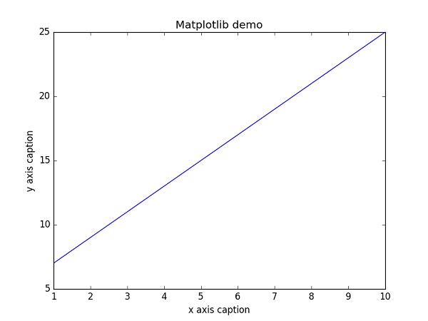
Instead of the linear graph, the values can be displayed discretely by adding a format string to the plot() function. Following formatting characters can be used.

Sr.No.	Character & Description
1	'-' Solid line style
2	'--' Dashed line style
3	'-.' Dash-dot line style
4	':' Dotted line style
5	'.' Point marker
6	',' Pixel marker
7	'o' Circle marker
8	'v' Triangle_down marker
9	'^' Triangle_up marker
10	'<' Triangle_left marker
11	'>' Triangle_right marker
12	'1' Tri_down marker
13	'2' Tri_up marker
14	'3' Tri_left marker
15	'4' Tri_right marker
16	's' Square marker
17	'p' Pentagon marker
18	'*' Star marker
19	'h' Hexagon1 marker
20	'H' Hexagon2 marker
21	'+' Plus marker
22	'x' X marker
23	'D' Diamond marker
24	'd' Thin_diamond marker
25	'\|' Vline marker
26	'_' Hline marker

The following color abbreviations are also defined.

Character	Color
'b'	Blue
'g'	Green
'r'	Red
'c'	Cyan
'm'	Magenta
'y'	Yellow
'k'	Black
'w'	White

To display the circles representing points, instead of the line in the above example, use “ob” as the format string in plot() function.

Example

import numpy as np 
from matplotlib import pyplot as plt 

x = np.arange(1,11) 
y = 2 * x + 5 
plt.title("Matplotlib demo") 
plt.xlabel("x axis caption") 
plt.ylabel("y axis caption") 
plt.plot(x,y,"ob") 
plt.show()

The above code should produce the following output −

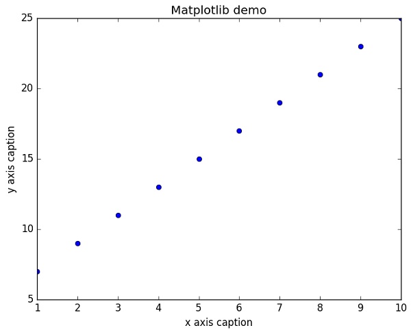
Sine Wave Plot

The following script produces the sine wave plot using matplotlib.

Example

import numpy as np 
import matplotlib.pyplot as plt  

# Compute the x and y coordinates for points on a sine curve 
x = np.arange(0, 3 * np.pi, 0.1) 
y = np.sin(x) 
plt.title("sine wave form") 

# Plot the points using matplotlib 
plt.plot(x, y) 
plt.show()

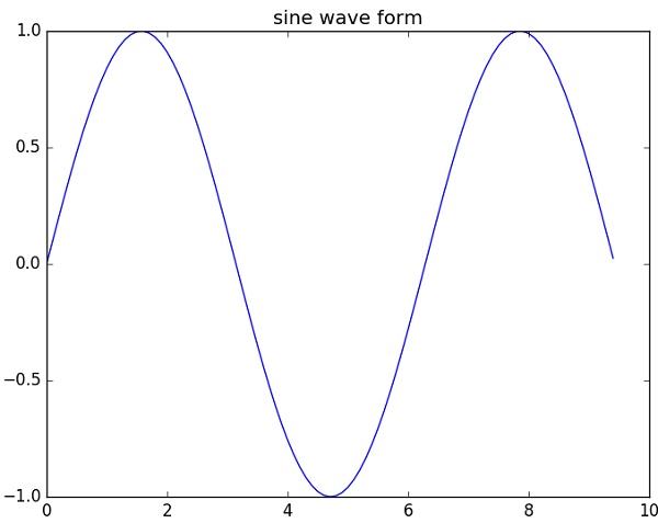
subplot()

The subplot() function allows you to plot different things in the same figure. In the following script, sine and cosine values are plotted.

Example

import numpy as np 
import matplotlib.pyplot as plt  
   
# Compute the x and y coordinates for points on sine and cosine curves 
x = np.arange(0, 3 * np.pi, 0.1) 
y_sin = np.sin(x) 
y_cos = np.cos(x)  
   
# Set up a subplot grid that has height 2 and width 1, 
# and set the first such subplot as active. 
plt.subplot(2, 1, 1)
   
# Make the first plot 
plt.plot(x, y_sin) 
plt.title('Sine')  
   
# Set the second subplot as active, and make the second plot. 
plt.subplot(2, 1, 2) 
plt.plot(x, y_cos) 
plt.title('Cosine')  
   
# Show the figure. 
plt.show()

The above code should produce the following output −

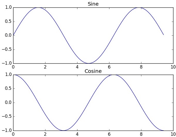
bar()

The pyplot submodule provides bar() function to generate bar graphs. The following example produces the bar graph of two sets of x and y arrays.

Example

from matplotlib import pyplot as plt 
x = [5,8,10] 
y = [12,16,6]  

x2 = [6,9,11] 
y2 = [6,15,7] 
plt.bar(x, y, align = 'center') 
plt.bar(x2, y2, color = 'g', align = 'center') 
plt.title('Bar graph') 
plt.ylabel('Y axis') 
plt.xlabel('X axis')  

plt.show()

This code should produce the following output −

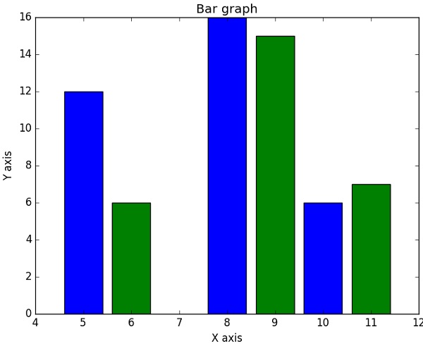
NumPy - Histogram Using Matplotlib

NumPy has a numpy.histogram() function that is a graphical representation of the frequency distribution of data. Rectangles of equal horizontal size corresponding to class interval called bin and variable height corresponding to frequency.

numpy.histogram()

The numpy.histogram() function takes the input array and bins as two parameters. The successive elements in bin array act as the boundary of each bin.

import numpy as np 
   
a = np.array([22,87,5,43,56,73,55,54,11,20,51,5,79,31,27]) 
np.histogram(a,bins = [0,20,40,60,80,100]) 
hist,bins = np.histogram(a,bins = [0,20,40,60,80,100]) 
print hist 
print bins

It will produce the following output −

[3 4 5 2 1]
[0 20 40 60 80 100]

plt()

Matplotlib can convert this numeric representation of histogram into a graph. The plt() function of pyplot submodule takes the array containing the data and bin array as parameters and converts into a histogram.

from matplotlib import pyplot as plt 
import numpy as np  
   
a = np.array([22,87,5,43,56,73,55,54,11,20,51,5,79,31,27]) 
plt.hist(a, bins = [0,20,40,60,80,100]) 
plt.title("histogram") 
plt.show()

It should produce the following output −

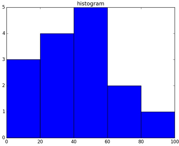
I/O with NumPy

The ndarray objects can be saved to and loaded from the disk files. The IO functions available are −

load() and save() functions handle /numPy binary files (with npyextension)
loadtxt() and savetxt() functions handle normal text files

NumPy introduces a simple file format for ndarray objects. This .npy file stores data, shape, dtype and other information required to reconstruct the ndarray in a disk file such that the array is correctly retrieved even if the file is on another machine with different architecture.

numpy.save()

The numpy.save() file stores the input array in a disk file with npyextension.

import numpy as np 
a = np.array([1,2,3,4,5]) 
np.save('outfile',a)

To reconstruct array from outfile.npy, use load() function.

import numpy as np 
b = np.load('outfile.npy') 
print b

It will produce the following output −

array([1, 2, 3, 4, 5])

The save() and load() functions accept an additional Boolean parameter allow_pickles. A pickle in Python is used to serialize and de-serialize objects before saving to or reading from a disk file.

savetxt()

The storage and retrieval of array data in simple text file format is done with savetxt() and loadtxt() functions.

Example

import numpy as np 

a = np.array([1,2,3,4,5]) 
np.savetxt('out.txt',a) 
b = np.loadtxt('out.txt') 
print b

It will produce the following output −

[ 1.  2.  3.  4.  5.]

The savetxt() and loadtxt() functions accept additional optional parameters such as header, footer, and delimiter.

Friday, July 20, 2018