Machine Learning with Python - Quick Guide
Python is a popular platform used for research and development of production systems. It is a vast language with number of modules, packages and libraries that provides multiple ways of achieving a task.
Python and its libraries like NumPy, SciPy, Scikit-Learn, Matplotlib are used in data science and data analysis. They are also extensively used for creating scalable machine learning algorithms. Python implements popular machine learning techniques such as Classification, Regression, Recommendation, and Clustering.
Python offers ready-made framework for performing data mining tasks on large volumes of data effectively in lesser time. It includes several implementations achieved through algorithms such as linear regression, logistic regression, Naïve Bayes, k-means, K nearest neighbor, and Random Forest.
Machine Learning with Python - Concepts
In this chapter, you will learn in detail about the concepts of Python in machine learning.
Python in Machine Learning
Python has libraries that enables developers to use optimized algorithms. It implements popular machine learning techniques such as recommendation, classification, and clustering. Therefore, it is necessary to have a brief introduction to machine learning before we move further.
What is Machine Learning?
Data science, machine learning and artificial intelligence are some of the top trending topics in the tech world today. Data mining and Bayesian analysis are trending and this is adding the demand for machine learning. This tutorial is your entry into the world of machine learning.
Machine learning is a discipline that deals with programming the systems so as to make them automatically learn and improve with experience. Here, learning implies recognizing and understanding the input data and taking informed decisions based on the supplied data. It is very difficult to consider all the decisions based on all possible inputs. To solve this problem, algorithms are developed that build knowledge from a specific data and past experience by applying the principles of statistical science, probability, logic, mathematical optimization, reinforcement learning, and control theory.
Applications of Machine Learning Algorithms
The developed machine learning algorithms are used in various applications such as −
- Vision processing
- Language processing
- Forecasting things like stock market trends, weather
- Pattern recognition
- Games
- Data mining
- Expert systems
- Robotics
Steps Involved in Machine Learning
A machine learning project involves the following steps −
- Defining a Problem
- Preparing Data
- Evaluating Algorithms
- Improving Results
- Presenting Results
The best way to get started using Python for machine learning is to work through a project end-to-end and cover the key steps like loading data, summarizing data, evaluating algorithms and making some predictions. This gives you a replicable method that can be used dataset after dataset. You can also add further data and improve the results.
Environment Setup
In this chapter, you will learn how to setup the working environment for Python machine learning on your local computer.
Libraries and Packages
To understand machine learning, you need to have basic knowledge of Python programming. In addition, there are a number of libraries and packages generally used in performing various machine learning tasks as listed below −
- numpy − is used for its N-dimensional array objects
- pandas − is a data analysis library that includes dataframes
- matplotlib − is 2D plotting library for creating graphs and plots
- scikit-learn − the algorithms used for data analysis and data mining tasks
- seaborn − a data visualization library based on matplotlib
Installation
You can install software for machine learning in any of the two methods as discussed here −
Method 1
Download and install Python separately from python.org on various operating systems as explained below −
To install Python after downloading, double click the .exe (for Windows) or .pkg (for Mac) file and follow the instructions on the screen.
For Linux OS, check if Python is already installed by using the following command at the prompt −
$ python --version. ...
If Python 2.7 or later is not installed, install Python with the distribution's package manager. Note that the command and package name varies.
On Debian derivatives such as Ubuntu, you can use apt −
$ sudo apt-get install python3
Now, open the command prompt and run the following command to verify that Python is installed correctly −
$ python3 --version

Python 3.6.2
Similarly, we can download and install necessary libraries like numpy, matplotlib etc. individually using installers like pip. For this purpose, you can use the commands shown here −
$pip install numpy
$pip install matplotlib
$pip install pandas
$pip install seaborn
Method 2
Alternatively, to install Python and other scientific computing and machine learning packages simultaneously, we should install Anaconda distribution. It is a Python implementation for Linux, Windows and OSX, and comprises various machine learning packages like numpy, scikit-learn, and matplotlib. It also includes Jupyter Notebook, an interactive Python environment. We can install Python 2.7 or any 3.x version as per our requirement.
To download the free Anaconda Python distribution from Continuum Analytics, you can do the following −
Visit the official site of Continuum Analytics and its download page. Note that the installation process may take 15-20 minutes as the installer contains Python, associated packages, a code editor, and some other files. Depending on your operating system, choose the installation process as explained here −
For Windows − Select the Anaconda for Windows section and look in the column with Python 2.7 or 3.x. You can find that there are two versions of the installer, one for 32-bit Windows, and one for 64-bit Windows. Choose the relevant one.
For Mac OS − Scroll to the Anaconda for OS X section. Look in the column with Python 2.7 or 3.x. Note that here there is only one version of the installer: the 64-bit version.
For Linux OS − We select the "Anaconda for Linux" section. Look in the column with Python 2.7 or 3.x.
Note that you have to ensure that Anaconda’s Python distribution installs into a single directory, and does not affect other Python installations, if any, on your system.
To work with graphs and plots, we will need these Python library packages - matplotlib and seaborn.
If you are using Anaconda Python, your system already has numpy, matplotlib, pandas, seaborn, etc. installed. We start the Anaconda Navigator to access either Jupyter Note book or Spyder IDE of python.
After opening either of them, type the following commands −
import numpy

import matplotlib
Now, we need to check if installation is successful. For this, go to the command line and type in the following command −
$ python
Python 3.6.3 |Anaconda custom (32-bit)| (default, Oct 13 2017, 14:21:34)
[GCC 7.2.0] on linux
Next, you can import the required libraries and print their versions as shown −
>>>import numpy
>>>print numpy.__version__
1.14.2

>>> import matplotlib
>>> print (matplotlib.__version__)
2.1.2

>> import pandas
>>> print (pandas.__version__)
0.22.0

>>> import seaborn
>>> print (seaborn.__version__)
0.8.1
Types of Learning
Machine Learning (ML) is an automated learning with little or no human intervention. It involves programming computers so that they learn from the available inputs. The main purpose of machine learning is to explore and construct algorithms that can learn from the previous data and make predictions on new input data.
The input to a learning algorithm is training data, representing experience, and the output is any expertise, which usually takes the form of another algorithm that can perform a task. The input data to a machine learning system can be numerical, textual, audio, visual, or multimedia. The corresponding output data of the system can be a floating-point number, for instance, the velocity of a rocket, an integer representing a category or a class, for example, a pigeon or a sunflower from image recognition.
In this chapter, we will learn about the training data our programs will access and how learning process is automated and how the success and performance of such machine learning algorithms is evaluated.
Concepts of Learning
Learning is the process of converting experience into expertise or knowledge.
Learning can be broadly classified into three categories, as mentioned below, based on the nature of the learning data and interaction between the learner and the environment.
- Supervised Learning
- Unsupervised Learning
- Semi-supervised Learning
Similarly, there are four categories of machine learning algorithms as shown below −
- Supervised learning algorithm
- Unsupervised learning algorithm
- Semi-supervised learning algorithm
- Reinforcement learning algorithm
However, the most commonly used ones are supervised and unsupervised learning.
Supervised Learning
Supervised learning is commonly used in real world applications, such as face and speech recognition, products or movie recommendations, and sales forecasting. Supervised learning can be further classified into two types - Regression and Classification.
Regression trains on and predicts a continuous-valued response, for example predicting real estate prices.
Classification attempts to find the appropriate class label, such as analyzing positive/negative sentiment, male and female persons, benign and malignant tumors, secure and unsecure loans etc.
In supervised learning, learning data comes with description, labels, targets or desired outputs and the objective is to find a general rule that maps inputs to outputs. This kind of learning data is called labeled data. The learned rule is then used to label new data with unknown outputs.
Supervised learning involves building a machine learning model that is based on labeled samples. For example, if we build a system to estimate the price of a plot of land or a house based on various features, such as size, location, and so on, we first need to create a database and label it. We need to teach the algorithm what features correspond to what prices. Based on this data, the algorithm will learn how to calculate the price of real estate using the values of the input features.
Supervised learning deals with learning a function from available training data. Here, a learning algorithm analyzes the training data and produces a derived function that can be used for mapping new examples. There are many supervised learning algorithms such as Logistic Regression, Neural networks, Support Vector Machines (SVMs), and Naive Bayes classifiers.
Common examples of supervised learning include classifying e-mails into spam and not-spam categories, labeling webpages based on their content, and voice recognition.
Unsupervised Learning
Unsupervised learning is used to detect anomalies, outliers, such as fraud or defective equipment, or to group customers with similar behaviors for a sales campaign. It is the opposite of supervised learning. There is no labeled data here.
When learning data contains only some indications without any description or labels, it is up to the coder or to the algorithm to find the structure of the underlying data, to discover hidden patterns, or to determine how to describe the data. This kind of learning data is called unlabeled data.
Suppose that we have a number of data points, and we want to classify them into several groups. We may not exactly know what the criteria of classification would be. So, an unsupervised learning algorithm tries to classify the given dataset into a certain number of groups in an optimum way.
Unsupervised learning algorithms are extremely powerful tools for analyzing data and for identifying patterns and trends. They are most commonly used for clustering similar input into logical groups. Unsupervised learning algorithms include Kmeans, Random Forests, Hierarchical clustering and so on.
Semi-supervised Learning
If some learning samples are labeled, but some other are not labeled, then it is semi-supervised learning. It makes use of a large amount of unlabeled data for training and a small amount of labeled data for testing. Semi-supervised learning is applied in cases where it is expensive to acquire a fully labeled dataset while more practical to label a small subset. For example, it often requires skilled experts to label certain remote sensing images, and lots of field experiments to locate oil at a particular location, while acquiring unlabeled data is relatively easy.
Reinforcement Learning
Here learning data gives feedback so that the system adjusts to dynamic conditions in order to achieve a certain objective. The system evaluates its performance based on the feedback responses and reacts accordingly. The best known instances include self-driving cars and chess master algorithm AlphaGo.
Purpose of Machine Learning
Machine learning can be seen as a branch of AI or Artificial Intelligence, since, the ability to change experience into expertise or to detect patterns in complex data is a mark of human or animal intelligence.
As a field of science, machine learning shares common concepts with other disciplines such as statistics, information theory, game theory, and optimization.
As a subfield of information technology, its objective is to program machines so that they will learn.
However, it is to be seen that, the purpose of machine learning is not building an automated duplication of intelligent behavior, but using the power of computers to complement and supplement human intelligence. For example, machine learning programs can scan and process huge databases detecting patterns that are beyond the scope of human perception.
Data Preprocessing, Analysis & Visualization
In the real world, we usually come across lots of raw data which is not fit to be readily processed by machine learning algorithms. We need to preprocess the raw data before it is fed into various machine learning algorithms. This chapter discusses various techniques for preprocessing data in Python machine learning.
Data Preprocessing
In this section, let us understand how we preprocess data in Python.
Initially, open a file with a .py extension, for example prefoo.py file, in a text editor like notepad.
Then, add the following piece of code to this file −
import numpy as np

from sklearn import preprocessing

#We imported a couple of packages. Let's create some sample data and add the line to this file:

input_data = np.array([[3, -1.5, 3, -6.4], [0, 3, -1.3, 4.1], [1, 2.3, -2.9, -4.3]])
We are now ready to operate on this data.
Preprocessing Techniques
Data can be preprocessed using several techniques as discussed here −
Mean removal
It involves removing the mean from each feature so that it is centered on zero. Mean removal helps in removing any bias from the features.
You can use the following code for mean removal −
data_standardized = preprocessing.scale(input_data)
print "\nMean = ", data_standardized.mean(axis = 0)
print "Std deviation = ", data_standardized.std(axis = 0)
Now run the following command on the terminal −
$ python prefoo.py
You can observe the following output −
Mean = [ 5.55111512e-17 -3.70074342e-17 0.00000000e+00 -1.85037171e-17]
Std deviation = [1. 1. 1. 1.]
Observe that in the output, mean is almost 0 and the standard deviation is 1.
Scaling
The values of every feature in a data point can vary between random values. So, it is important to scale them so that this matches specified rules.
You can use the following code for scaling −
data_scaler = preprocessing.MinMaxScaler(feature_range = (0, 1))
data_scaled = data_scaler.fit_transform(input_data)
print "\nMin max scaled data = ", data_scaled
Now run the code and you can observe the following output −
Min max scaled data = [ [ 1. 0. 1. 0. ]
                        [ 0. 1. 0.27118644 1. ]
                        [ 0.33333333 0.84444444 0. 0.2 ]
]
Note that all the values have been scaled between the given range.
Normalization
Normalization involves adjusting the values in the feature vector so as to measure them on a common scale. Here, the values of a feature vector are adjusted so that they sum up to 1. We add the following lines to the prefoo.py file −
You can use the following code for normalization −
data_normalized = preprocessing.normalize(input_data, norm  = 'l1')
print "\nL1 normalized data = ", data_normalized
Now run the code and you can observe the following output −
L1 normalized data = [  [ 0.21582734 -0.10791367 0.21582734 -0.46043165]
                        [ 0. 0.35714286 -0.1547619 0.48809524]
                        [ 0.0952381 0.21904762 -0.27619048 -0.40952381]
]
Normalization is used to ensure that data points do not get boosted due to the nature of their features.
Binarization
Binarization is used to convert a numerical feature vector into a Boolean vector. You can use the following code for binarization −
data_binarized = preprocessing.Binarizer(threshold=1.4).transform(input_data)
print "\nBinarized data =", data_binarized
Now run the code and you can observe the following output −
Binarized data = [[ 1. 0. 1. 0.]
                  [ 0. 1. 0. 1.]
                  [ 0. 1. 0. 0.]
                 ]
This technique is helpful when we have prior knowledge of the data.
One Hot Encoding
It may be required to deal with numerical values that are few and scattered, and you may not need to store these values. In such situations you can use One Hot Encoding technique.
If the number of distinct values is k, it will transform the feature into a k-dimensional vector where only one value is 1 and all other values are 0.
You can use the following code for one hot encoding −
encoder = preprocessing.OneHotEncoder()
encoder.fit([  [0, 2, 1, 12],
               [1, 3, 5, 3],
               [2, 3, 2, 12],
               [1, 2, 4, 3]
])
encoded_vector = encoder.transform([[2, 3, 5, 3]]).toarray()
print "\nEncoded vector =", encoded_vector
Now run the code and you can observe the following output −
Encoded vector = [[ 0. 0. 1. 0. 1. 0. 0. 0. 1. 1. 0.]]
In the example above, let us consider the third feature in each feature vector. The values are 1, 5, 2, and 4.
There are four separate values here, which means the one-hot encoded vector will be of length 4. If we want to encode the value 5, it will be a vector [0, 1, 0, 0]. Only one value can be 1 in this vector. The second element is 1, which indicates that the value is 5.
Label Encoding
In supervised learning, we mostly come across a variety of labels which can be in the form of numbers or words. If they are numbers, then they can be used directly by the algorithm. However, many times, labels need to be in readable form. Hence, the training data is usually labelled with words.
Label encoding refers to changing the word labels into numbers so that the algorithms can understand how to work on them. Let us understand in detail how to perform label encoding −
Create a new Python file, and import the preprocessing package −
from sklearn import preprocessing
label_encoder = preprocessing.LabelEncoder()
input_classes = ['suzuki', 'ford', 'suzuki', 'toyota', 'ford', 'bmw']
label_encoder.fit(input_classes)
print "\nClass mapping:"
for i, item in enumerate(label_encoder.classes_):
print item, '-->', i
Now run the code and you can observe the following output −
Class mapping:
bmw --> 0
ford --> 1
suzuki --> 2
toyota --> 3
As shown in above output, the words have been changed into 0-indexed numbers. Now, when we deal with a set of labels, we can transform them as follows −
labels = ['toyota', 'ford', 'suzuki']
encoded_labels = label_encoder.transform(labels)
print "\nLabels =", labels
print "Encoded labels =", list(encoded_labels)
Now run the code and you can observe the following output −
Labels = ['toyota', 'ford', 'suzuki']
Encoded labels = [3, 1, 2]
This is efficient than manually maintaining mapping between words and numbers. You can check by transforming numbers back to word labels as shown in the code here −
encoded_labels = [3, 2, 0, 2, 1]
decoded_labels = label_encoder.inverse_transform(encoded_labels)
print "\nEncoded labels =", encoded_labels
print "Decoded labels =", list(decoded_labels)
Now run the code and you can observe the following output −
Encoded labels = [3, 2, 0, 2, 1]
Decoded labels = ['toyota', 'suzuki', 'bmw', 'suzuki', 'ford']
From the output, you can observe that the mapping is preserved perfectly.
Data Analysis
This section discusses data analysis in Python machine learning in detail −
Loading the Dataset
We can load the data directly from the UCI Machine Learning repository. Note that here we are using pandas to load the data. We will also use pandas next to explore the data both with descriptive statistics and data visualization. Observe the following code and note that we are specifying the names of each column when loading the data.
import pandas
data = ‘pima_indians.csv’
names = ['Pregnancies', 'Glucose', 'BloodPressure', 'SkinThickness', 'Insulin', ‘Outcome’]
dataset = pandas.read_csv(data, names = names)
When you run the code, you can observe that the dataset loads and is ready to be analyzed. Here, we have downloaded the pima_indians.csv file and moved it into our working directory and loaded it using the local file name.
Summarizing the Dataset
Summarizing the data can be done in many ways as follows −
- Check dimensions of the dataset
- List the entire data
- View the statistical summary of all attributes
- Breakdown of the data by the class variable
Dimensions of Dataset
You can use the following command to check how many instances (rows) and attributes (columns) the data contains with the shape property.
print(dataset.shape)
Then, for the code that we have discussed, we can see 769 instances and 6 attributes −
(769, 6)
List the Entire Data
You can view the entire data and understand its summary −
print(dataset.head(20))
This command prints the first 20 rows of the data as shown −
Sno Pregnancies Glucose BloodPressure SkinThickness Insulin Outcome
1        6        148         72           35          0       1
2        1         85         66           29          0       0
3        8        183         64            0          0       1
4        1         89         66           23         94       0
5        0        137         40           35        168       1
6        5        116         74            0          0       0
7        3         78         50           32         88       1
8       10        115          0            0          0       0
9        2        197         70           45        543       1
10       8        125         96            0          0       1
11       4        110         92            0          0       0
12      10        168         74            0          0       1
13      10        139         80            0          0       0
14       1        189         60           23        846       1
15       5        166         72           19        175       1
16       7        100          0            0          0       1
17       0        118         84           47        230       1
18       7        107         74            0          0       1
19       1        103         30           38         83       0
View the Statistical Summary
You can view the statistical summary of each attribute, which includes the count, unique, top and freq, by using the following command.
print(dataset.describe())
The above command gives you the following output that shows the statistical summary of each attribute −
         Pregnancies Glucose BloodPressur SkinThckns Insulin Outcome
count       769       769       769         769       769     769
unique       18       137        48          52       187       3
top           1       100        70           0         0       0
freq        135        17        57         227       374     500
Breakdown the Data by Class Variable
You can also look at the number of instances (rows) that belong to each outcome as an absolute count, using the command shown here −
print(dataset.groupby('Outcome').size())
Then you can see the number of outcomes of instances as shown −
Outcome
0         500
1         268
Outcome     1
dtype: int64
Data Visualization
You can visualize data using two types of plots as shown −
- Univariate plots to understand each attribute
- Multivariate plots to understand the relationships between attributes
Univariate Plots
Univariate plots are plots of each individual variable. Consider a case where the input variables are numeric, and we need to create box and whisker plots of each. You can use the following code for this purpose.
import pandas
import matplotlib.pyplot as plt
data = 'iris_df.csv'
names = ['sepal-length', 'sepal-width', 'petal-length', 'petal-width', 'class']
dataset = pandas.read_csv(data, names=names)
dataset.plot(kind='box', subplots=True, layout=(2,2), sharex=False, sharey=False)
plt.show()
You can see the output with a clearer idea of the distribution of the input attributes as shown −
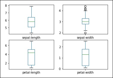
Box and Whisker Plots
You can create a histogram of each input variable to get an idea of the distribution using the commands shown below −
#histograms
dataset.hist()
plt().show()
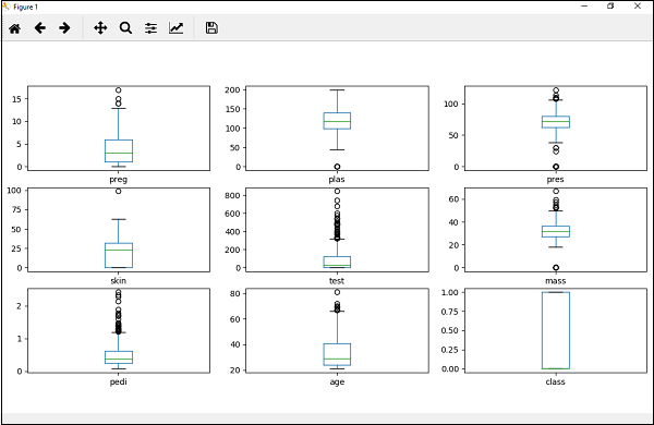
From the output, you can see that two of the input variables have a Gaussian distribution. Thus these plots help in giving an idea about the algorithms that we can use in our program.
Multivariate Plots
Multivariate plots help us to understand the interactions between the variables.
Scatter Plot Matrix
First, let’s look at scatterplots of all pairs of attributes. This can be helpful to spot structured relationships between input variables.
from pandas.plotting import scatter_matrix
scatter_matrix(dataset)
plt.show()
You can observe the output as shown −
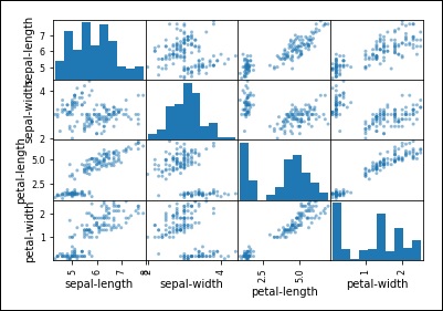
Observe that in the output there is a diagonal grouping of some pairs of attributes. This indicates a high correlation and a predictable relationship.
Training Data and Test Data
Training data and test data are two important concepts in machine learning. This chapter discusses them in detail.
Training Data
The observations in the training set form the experience that the algorithm uses to learn. In supervised learning problems, each observation consists of an observed output variable and one or more observed input variables.
Test Data
The test set is a set of observations used to evaluate the performance of the model using some performance metric. It is important that no observations from the training set are included in the test set. If the test set does contain examples from the training set, it will be difficult to assess whether the algorithm has learned to generalize from the training set or has simply memorized it.
A program that generalizes well will be able to effectively perform a task with new data. In contrast, a program that memorizes the training data by learning an overly complex model could predict the values of the response variable for the training set accurately, but will fail to predict the value of the response variable for new examples. Memorizing the training set is called over-fitting. A program that memorizes its observations may not perform its task well, as it could memorize relations and structures that are noise or coincidence. Balancing memorization and generalization, or over-fitting and under-fitting, is a problem common to many machine learning algorithms. Regularizationmay be applied to many models to reduce over-fitting.
In addition to the training and test data, a third set of observations, called a validation or hold-out set, is sometimes required. The validation set is used to tune variables called hyper parameters, which control how the model is learned. The program is still evaluated on the test set to provide an estimate of its performance in the real world; its performance on the validation set should not be used as an estimate of the model's real-world performance since the program has been tuned specifically to the validation data. It is common to partition a single set of supervised observations into training, validation, and test sets. There are no requirements for the sizes of the partitions, and they may vary according to the amount of data available. It is common to allocate 50 percent or more of the data to the training set, 25 percent to the test set, and the remainder to the validation set.
Some training sets may contain only a few hundred observations; others may include millions. Inexpensive storage, increased network connectivity, the ubiquity of sensor-packed smartphones, and shifting attitudes towards privacy have contributed to the contemporary state of big data, or training sets with millions or billions of examples.
However, machine learning algorithms also follow the maxim "garbage in, garbage out." A student who studies for a test by reading a large, confusing textbook that contains many errors will likely not score better than a student who reads a short but well-written textbook. Similarly, an algorithm trained on a large collection of noisy, irrelevant, or incorrectly labeled data will not perform better than an algorithm trained on a smaller set of data that is more representative of problems in the real world.
Many supervised training sets are prepared manually, or by semi-automated processes. Creating a large collection of supervised data can be costly in some domains. Fortunately, several datasets are bundled with scikit-learn, allowing developers to focus on experimenting with models instead.
During development, and particularly when training data is scarce, a practice called cross-validation can be used to train and validate an algorithm on the same data. In cross-validation, the training data is partitioned. The algorithm is trained using all but one of the partitions, and tested on the remaining partition. The partitions are then rotated several times so that the algorithm is trained and evaluated on all of the data.
Consider for example that the original dataset is partitioned into five subsets of equal size, labeled A through E. Initially, the model is trained on partitions B through E, and tested on partition A. In the next iteration, the model is trained on partitions A, C, D, and E, and tested on partition B. The partitions are rotated until models have been trained and tested on all of the partitions. Cross-validation provides a more accurate estimate of the model's performance than testing a single partition of the data.
Performance Measures − Bias and Variance
Many metrics can be used to measure whether or not a program is learning to perform its task more effectively. For supervised learning problems, many performance metrics measure the number of prediction errors.
There are two fundamental causes of prediction error for a model -bias and variance. Assume that you have many training sets that are all unique, but equally representative of the population. A model with a high bias will produce similar errors for an input regardless of the training set it was trained with; the model biases its own assumptions about the real relationship over the relationship demonstrated in the training data. A model with high variance, conversely, will produce different errors for an input depending on the training set that it was trained with. A model with high bias is inflexible, but a model with high variance may be so flexible that it models the noise in the training set. That is, a model with high variance over-fits the training data, while a model with high bias under-fits the training data.
Ideally, a model will have both low bias and variance, but efforts to decrease one will frequently increase the other. This is known as the bias-variance trade-off. We may have to consider the bias-variance tradeoffs of several models introduced in this tutorial. Unsupervised learning problems do not have an error signal to measure; instead, performance metrics for unsupervised learning problems measure some attributes of the structure discovered in the data. Most performance measures can only be worked out for a specific type of task.
Machine learning systems should be evaluated using performance measures that represent the costs of making errors in the real world. While this looks trivial, the following example illustrates the use of a performance measure that is right for the task in general but not for its specific application.
Accuracy, Precision and Recall
Consider a classification task in which a machine learning system observes tumors and has to predict whether these tumors are benign or malignant. Accuracy, or the fraction of instances that were classified correctly, is an obvious measure of the program's performance. While accuracy does measure the program's performance, it does not make distinction between malignant tumors that were classified as being benign, and benign tumors that were classified as being malignant. In some applications, the costs incurred on all types of errors may be the same. In this problem, however, failing to identify malignant tumors is a more serious error than classifying benign tumors as being malignant by mistake.
We can measure each of the possible prediction outcomes to create different snapshots of the classifier's performance. When the system correctly classifies a tumor as being malignant, the prediction is called a true positive. When the system incorrectly classifies a benign tumor as being malignant, the prediction is a false positive. Similarly, a false negative is an incorrect prediction that the tumor is benign, and a true negative is a correct prediction that a tumor is benign. These four outcomes can be used to calculate several common measures of classification performance, like accuracy, precision, recall and so on.
Accuracy is calculated with the following formula −
ACC = (TP + TN)/(TP + TN + FP + FN)
Where, TP is the number of true positives
TN is the number of true negatives
FP is the number of false positives
FN is the number of false negatives.
Precision is the fraction of the tumors that were predicted to be malignant that are actually malignant. Precision is calculated with the following formula −
PREC = TP/(TP + FP)
Recall is the fraction of malignant tumors that the system identified. Recall is calculated with the following formula −
R = TP/(TP + FN)
In this example, precision measures the fraction of tumors that were predicted to be malignant that are actually malignant. Recall measures the fraction of truly malignant tumors that were detected. The precision and recall measures could reveal that a classifier with impressive accuracy actually fails to detect most of the malignant tumors. If most tumors are benign, even a classifier that never predicts malignancy could have high accuracy. A different classifier with lower accuracy and higher recall might be better suited to the task, since it will detect more of the malignant tumors. Many other performance measures for classification can also be used.
Machine Learning with Python - Techniques
This chapter discusses each of the techniques used in machine learning in detail.
Classification
Classification is a machine learning technique that uses known data to determine how the new data should be classified into a set of existing categories.
Consider the following examples to understand classification technique −
A credit card company receives tens of thousands of applications for new credit cards. These applications contain information about several different features like age, location, sex, annual salary, credit record etc. The task of the algorithm here is to classify the card applicants into categories like those who have good credit record, bad credit record and those who have a mixed credit record.
In a hospital, the emergency room has more than 15 features (age, blood pressure, heart condition, severity of ailment etc.) to analyze before deciding whether a given patient has to be put in an intensive care unit as it is a costly proposition and only those patients who can survive and afford the cost are given top priority. The problem here is to classify the patients into high risk and low risk patients based on the available features or parameters.
While classifying a given set of data, the classifier system performs the following actions −
- Initially a new data model is prepared using any of the learning algorithms.
- Then the prepared data model is tested.
- Later, this data model is used to examine the new data and to determine its class.
Classification, also called categorization, is a machine learning technique that uses known data to determine how the new data should be classified into a set of existing labels/classes/categories.
In classification tasks, the program must learn to predict discrete values for the dependent or output variables from one or more independent or input variables. That is, the program must predict the most probable class, category or label for new observations. Applications of classification include predicting whether on a day it will rain or not, or predicting if a certain company’s share price will rise or fall, or deciding if an article belongs to the sports or entertainment section.
Classification is a form of supervised learning. Mail service providers like Gmail, Yahoo and others use this technique to classify a new mail as spam or not spam. The classification algorithm trains itself by analyzing user behavior of marking certain mails as spams. Based on that information, the classifier decides whether a new mail should go into the inbox or into the spam folder.
Applications of Classification
- Detection of Credit card fraud - The Classification method is used to predict credit card frauds. Employing historical records of previous frauds, the classifier can predict which future transactions may turn into frauds.
- E-mail spam - Depending on the features of previous spam mails, the classifier determines whether a newly received e-mail should be sent to the spam folder.
Naive Bayes Classifier Technique
Classification techniques include Naive Bayes Classifier, which is a simple technique for constructing classifiers. It is not one algorithm for training such classifiers, but a group of algorithms. A Bayes classifier constructs models to classify problem instances. These classifications are made using the available data.
An important feature of naive Bayes classifier is that it only requires a small amount of training data to estimate the parameters necessary for classification. For some types of models, naive Bayes classifiers can be trained very efficiently in a supervised learning setting.
In spite of its oversimplified assumptions, naive Bayes classifiers have worked efficiently in many complex real-world situations. These have worked well in spam filtering and document classification.
Regression
In regression, the program predicts the value of a continuous output or response variable. Examples of regression problems include predicting the sales for a new product, or the salary for a job based on its description. Similar to classification, regression problems require supervised learning. In regression tasks, the program predicts the value of a continuous output or response variable from the input or explanatory variables.
Recommendation
Recommendation is a popular method that provides close recommendations based on user information such as history of purchases, clicks, and ratings. Google and Amazon use this method to display a list of recommended items for their users, based on the information from their past actions. There are recommender engines that work in the background to capture user behavior and recommend selected items based on earlier user actions. Facebook also uses the recommender method to identify and recommend people and send friend suggestions to its users.
A recommendation engine is a model that predicts what a user may be interested in based on his past record and behavior. When this is applied in the context of movies, this becomes a movie-recommendation engine. We filter items in the movie database by predicting how a user might rate them. This helps us in connecting the users with the right content from the movie database. This technique is useful in two ways: If we have a massive database of movies, the user may or may not find content relevant to his choices. Also, by recommending the relevant content, we can increase consumption and get more users.
Netflix, Amazon Prime and similar movie rental companies rely heavily on recommendation engines to keep their users engaged. Recommendation engines usually produce a list of recommendations using either collaborative filtering or content-based filtering. The difference between the two types is in the way the recommendations are extracted. Collaborative filtering constructs a model from the past behavior of the current user as well as ratings given by other users. This model then is used to predict what this user might be interested in. Content-based filtering, on the other hand, uses the features of the item itself in order to recommend more items to the user. The similarity between items is the main motivation here. Collaborative filtering is often used more in such recommendation methods.
Clustering
Groups of related observations are called clusters. A common unsupervised learning task is to find clusters within the training data.
We can also define clustering as a procedure to organize items of a given collection into groups based on some similar features. For example, online news publishers group their news articles using clustering.
Applications of Clustering
Clustering finds applications in many fields such market research, pattern recognition, data analysis, and image processing.as discussed here −
- Helps marketers to discover distinct groups in their customer basis and characterize their customer groups based on purchasing patterns.
- In biology, it can be used to derive plant and animal taxonomies, categorize genes with similar functionality and gain insight into structures inherent in populations.
- Helps in identification of areas of similar land use in an earth observation database.
- Helps in classifying documents on the web for information discovery.
- Used in outlier detection applications such as detection of credit card fraud.
- Cluster Analysis serves as a data mining function tool to gain insight into the distribution of data to observe characteristics of each cluster.
The task, called clustering or cluster analysis, assigns observations to groups such that observations within groups are more similar to each other based on some similarity measure than they are to observations in other groups.
Clustering is often used to explore a dataset. For example, given a collection of movie reviews, a clustering algorithm might discover sets of positive and negative reviews. The system will not be able to label the clusters as "positive" or "negative"; without supervision, it will only have knowledge that the grouped observations are similar to each other by some measure. A common application of clustering is discovering segments of customers within a market for a product. By understanding what attributes are common to particular groups of customers, marketers can decide what aspects of their campaigns need to be emphasized. Clustering is also used by Internet radio services; for example, given a collection of songs, a clustering algorithm might be able to group the songs according to their genres. Using different similarity measures, the same clustering algorithm might group the songs by their keys, or by the instruments they contain.
Unsupervised learning tasks include clustering, in which observations are organized into groups according to some similar feature. Clustering is used to form groups or clusters of similar data based on common characteristics.
Clustering is a form of unsupervised learning. Search engines such as Google, Bing and Yahoo! use clustering techniques to group data with similar characteristics. Newsgroups use clustering techniques to group various articles based on related topics.
The clustering engine goes through the input data completely and based on the characteristics of the data, it will decide under which cluster it should be grouped. The following points may be noted while clustering −
- A suitable clustering algorithm, is to be selected to group the elements of a cluster.
- A rule is required to verify the similarity between the newly encountered elements and the elements in the groups.
- A stopping condition is required to define the point where no clustering is required.
Types of Clustering
There are two types of clustering - flat clustering and hierarchical clustering.
Flat clustering creates a flat set of clusters without any clear structure that can relate clusters to each other. Hierarchical clustering creates a hierarchy of clusters. Hierarchical clustering gives a hierarchy of clusters as output, a structure that yields more information than the unstructured set of clusters returned by flat clustering. Hierarchical clustering does not require us to specify beforehand the number of clusters. The advantages of hierarchical clustering come at the cost of lower efficiency.
In general, we select flat clustering when efficiency is important and hierarchical clustering when one of the potential problems of flat clustering is an issue. Moreover, it is believed by many researchers that hierarchical clustering produces better clusters than flat clustering.
Clustering Algorithms
You need clustering algorithms to cluster a given data. Two algorithms are frequently used - Canopy clustering and K-Means clustering.
The canopy clustering algorithm is an unsupervised pre-clustering algorithm that is often used as preprocessing step for the K-means algorithm or the Hierarchical clustering algorithm. It is used to speed up clustering operations on large data sets, where using another algorithm directly may not be possible due to large size of the data sets.
K-means clustering is an important clustering algorithm. The k in k-means clustering algorithm represents the number of clusters the data is to be divided into. For example, if the k value specified in the algorithm is 3, then algorithm will divide the data into 3 clusters.
Each object is represented as a vector in space. Initially k points are chosen by the algorithm randomly and treated as centers, every object closest to each center are clustered. The k-means algorithm requires vector files as input, therefore we need to create vector files. After creating vectors, we proceed with k-means algorithm.
Machine Learning with Python - Algorithms
Machine learning algorithms can be broadly classified into two types - Supervised and Unsupervised. This chapter discusses them in detail.
Supervised Learning
This algorithm consists of a target or outcome or dependent variable which is predicted from a given set of predictor or independent variables. Using these set of variables, we generate a function that maps input variables to desired output variables. The training process continues until the model achieves a desired level of accuracy on the training data.
Examples of Supervised Learning - Regression, Decision Tree, Random Forest, KNN, Logistic Regression etc.
Unsupervised Learning
In this algorithm, there is no target or outcome or dependent variable to predict or estimate. It is used for clustering a given data set into different groups, which is widely used for segmenting customers into different groups for specific intervention. Apriori algorithm and K-means are some of the examples of Unsupervised Learning.
Reinforcement Learning
Using this algorithm, the machine is trained to make specific decisions. Here, the algorithm trains itself continually by using trial and error methods and feedback methods. This machine learns from past experiences and tries to capture the best possible knowledge to make accurate business decisions.
Markov Decision Process is an example of Reinforcement Learning.
List of Common Machine Learning Algorithms
Here is the list of commonly used machine learning algorithms that can be applied to almost any data problem −
- Linear Regression
- Logistic Regression
- Decision Tree
- SVM
- Naive Bayes
- KNN
- K-Means
- Random Forest
- Dimensionality Reduction Algorithms
- Gradient Boosting algorithms like GBM, XGBoost, LightGBM and CatBoost
This section discusses each of them in detail −
Linear Regression
Linear regression is used to estimate real world values like cost of houses, number of calls, total sales etc. based on continuous variable(s). Here, we establish relationship between dependent and independent variables by fitting a best line. This line of best fit is known as regression line and is represented by the linear equation Y= a *X + b.
In this equation −
Y – Dependent Variable
a – Slope
X – Independent variable
b – Intercept
These coefficients a and b are derived based on minimizing the sum of squared difference of distance between data points and regression line.
Example
The best way to understand linear regression is by considering an example. Suppose we are asked to arrange students in a class in the increasing order of their weights. By looking at the students and visually analyzing their heights and builds we can arrange them as required using a combination of these parameters, namely height and build. This is real world linear regression example. We have figured out that height and build have correlation to the weight by a relationship, which looks similar to the equation above.
Types of Linear Regression
Linear Regression is of mainly two types - Simple Linear Regression and Multiple Linear Regression. Simple Linear Regression is characterized by one independent variable while Multiple Linear Regression is characterized by more than one independent variables. While finding the line of best fit, you can fit a polynomial or curvilinear regression. You can use the following code for this purpose.
import matplotlib.pyplot as plt
plt.scatter(X, Y)

yfit = [a + b * xi for xi in X]
plt.plot(X, yfit)
Building a Linear Regressor
Regression is the process of estimating the relationship between input data and the continuous-valued output data. This data is usually in the form of real numbers, and our goal is to estimate the underlying function that governs the mapping from the input to the output.
Consider a mapping between input and output as shown −
1 --> 2
3 --> 6
4.3 --> 8.6
7.1 --> 14.2
You can easily estimate the relationship between the inputs and the outputs by analyzing the pattern. We can observe that the output is twice the input value in each case, hence the transformation would be − f(x) = 2x
Linear regression refers to estimating the relevant function using a linear combination of input variables. The preceding example was an example that consisted of one input variable and one output variable.
The goal of linear regression is to extract the relevant linear model that relates the input variable to the output variable. This aims to minimize the sum of squares of differences between the actual output and the predicted output using a linear function. This method is called Ordinary Least Squares. You may assume that a curvy line out there that fits these points better, but linear regression does not allow this. The main advantage of linear regression is that it is not complex. You may also find more accurate models in non-linear regression, but they will be slower. Here the model tries to approximate the input data points using a straight line.
Let us understand how to build a linear regression model in Python.
Consider that you have been provided with a data file, called data_singlevar.txt. This contains comma-separated lines where the first element is the input value and the second element is the output value that corresponds to this input value. You should use this as the input argument −
Assuming line of best fit for a set of points is −
y = a + b * x
where b = ( sum(xi * yi) - n * xbar * ybar ) / sum((xi - xbar)^2)
a = ybar - b * xbar
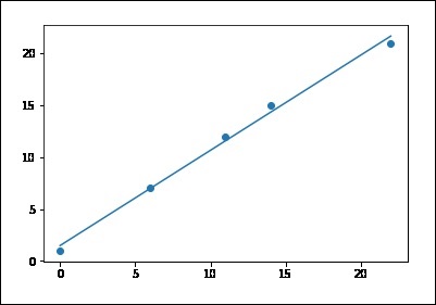
Use the following code for this purpose −
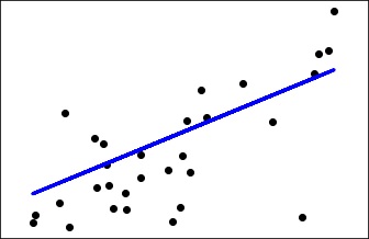
# sample points
X = [0, 6, 11, 14, 22]
Y = [1, 7, 12, 15, 21]

# solve for a and b
def best_fit(X, Y):
   xbar = sum(X)/len(X)
   ybar = sum(Y)/len(Y)
   n = len(X) # or len(Y)

   numer = sum([xi*yi for xi,yi in zip(X, Y)]) - n * xbar * ybar
   denum = sum([xi**2 for xi in X]) - n * xbar**2

   b = numer / denum
   a = ybar - b * xbar

   print('best fit line:\ny = {:.2f} + {:.2f}x'.format(a, b))

   return a, b

# solution
a, b = best_fit(X, Y)
#best fit line:
#y = 0.80 + 0.92x

# plot points and fit line
import matplotlib.pyplot as plt
plt.scatter(X, Y)
yfit = [a + b * xi for xi in X]
plt.plot(X, yfit)
plt.show()
best fit line:
y = 1.48 + 0.92x
If you run the above code, you can observe the output graph as shown −
Note that this example uses only the first feature of the diabetes dataset, in order to illustrate a two-dimensional plot of this regression technique. The straight line can be seen in the plot, showing how linear regression attempts to draw a straight line that will best minimize the residual sum of squares between the observed responses in the dataset, and the responses predicted by the linear approximation.
You can calculate the coefficients, the residual sum of squares and the variance score using the program code shown below −
import matplotlib.pyplot as plt
import numpy as np
from sklearn import datasets, linear_model
from sklearn.metrics import mean_squared_error, r2_score
# Load the diabetes dataset
diabetes = datasets.load_diabetes()
# Use only one feature
diabetes_X = diabetes.data[:, np.newaxis, 2]
# Split the data into training/testing sets
diabetes_X_train = diabetes_X[:-30]
diabetes_X_test = diabetes_X[-30:]

# Split the targets into training/testing sets
diabetes_y_train = diabetes.target[:-30]
diabetes_y_test = diabetes.target[-30:]
# Create linear regression object
regr = linear_model.LinearRegression()
# Train the model using the training sets
regr.fit(diabetes_X_train, diabetes_y_train)
# Make predictions using the testing set
diabetes_y_pred = regr.predict(diabetes_X_test)
# The coefficients
print('Coefficients: \n', regr.coef_)

# The mean squared error
print("Mean squared error: %.2f"
      % mean_squared_error(diabetes_y_test, diabetes_y_pred))
# Explained variance score: 1 is perfect prediction
print('Variance score: %.2f' % r2_score(diabetes_y_test, diabetes_y_pred))

# Plot outputs
plt.scatter(diabetes_X_test, diabetes_y_test, color = 'black')
plt.plot(diabetes_X_test, diabetes_y_pred, color = 'blue', linewidth = 3)
plt.xticks(())
plt.yticks(())
plt.show()
You can observe the following output once you execute the code given above −
Automatically created module for IPython interactive environment
('Coefficients: \n', array([ 941.43097333]))
Mean squared error: 3035.06
Variance score: 0.41
Logistic Regression
Logistic regression is another technique borrowed by machine learning from statistics. It is the preferred method for binary classification problems, that is, problems with two class values.
It is a classification algorithm and not a regression algorithm as the name says. It is used to estimate discrete values or values like 0/1, Y/N, T/F based on the given set of independent variable(s). It predicts the probability of occurrence of an event by fitting data to a logit function. Hence, it is also called logit regression. Since, it predicts the probability, its output values lie between 0 and 1.
Example
Let us understand this algorithm through a simple example.
Assume that there is a puzzle to solve that has only 2 outcome scenarios – either there is a solution or there is none. Now suppose, we have a wide range of puzzles to test a person which subjects he is good at. The outcomes may be something like this – if a trigonometry puzzle is given, a person may be 80% likely to solve it. On the other hand, if a geography puzzle is given, the person may be only 20% likely to solve it. This is where Logistic Regression helps in solving. As per math, the log odds of the outcome is expressed as a linear combination of the predictor variables.
odds = p/ (1-p) = probability of event occurrence / probability of not event occurrence

ln(odds) = ln(p/(1-p)) ; ln is the logarithm to the base ‘e’.
logit(p) = ln(p/(1-p)) = b0+b1X1+b2X2+b3X3....+bkXk
Note that in the above p is the probability of presence of the characteristic of interest. It chooses parameters that maximize the likelihood of observing the sample values rather than that minimize the sum of squared errors (like in ordinary regression).
Note that taking a log is one of the best mathematical way to replicate a step function.
The following points may be note-worthy when working on logistic regression −
- It is similar to regression in that the objective is to find the values for the coefficients that weigh each input variable.
- Unlike in linear regression, the prediction for the output is found using a non-linear function called the logistic function.
- The logistic function appears like a big ‘S’ and will change any value into the range 0 to 1. This is useful because we can apply a rule to the output of the logistic function to assign values to 0 and 1 and predict a class value.
- The way the logistic regression model is learned, the predictions made by it can also be used as the probability of a given data instance belonging to class 0 or class 1. This can be useful for problems where you need to give more reasoning for a prediction.
- Like linear regression, logistic regression works better when unrelated attributes of output variable are removed and similar attributes are removed.
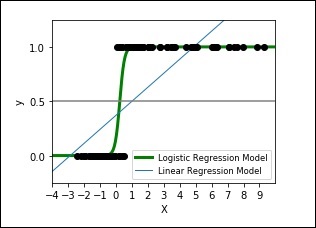
The following code shows how to develop a plot for logistic expression where a synthetic dataset is classified into values as either 0 or 1, that is class one or two, using the logistic curve.
import numpy as np
import matplotlib.pyplot as plt
from sklearn import linear_model
# This is the test set, it's a straight line with some Gaussian noise
xmin, xmax = -10, 10
n_samples = 100
np.random.seed(0)
X = np.random.normal(size = n_samples)
y = (X > 0).astype(np.float)
X[X > 0] *= 4
X += .3 * np.random.normal(size = n_samples)
X = X[:, np.newaxis]

# run the classifier
clf = linear_model.LogisticRegression(C=1e5)
clf.fit(X, y)

# and plot the result
plt.figure(1, figsize = (4, 3))
plt.clf()
plt.scatter(X.ravel(), y, color='black', zorder=20)
X_test = np.linspace(-10, 10, 300)
def model(x):
return 1 / (1 + np.exp(-x))
loss = model(X_test * clf.coef_ + clf.intercept_).ravel()
plt.plot(X_test, loss, color='blue', linewidth=3)
ols = linear_model.LinearRegression()
ols.fit(X, y)
plt.plot(X_test, ols.coef_ * X_test + ols.intercept_, linewidth=1)
plt.axhline(.5, color='.5')
plt.ylabel('y')
plt.xlabel('X')
plt.xticks(range(-10, 10))
plt.yticks([0, 0.5, 1])
plt.ylim(-.25, 1.25)
plt.xlim(-4, 10)
plt.legend(('Logistic Regression Model', 'Linear Regression Model'),
loc="lower right", fontsize='small')
plt.show()
The output plot will look like as shown here −
Decision Tree Algorithm
It is a supervised learning algorithm that is mostly used for classification problems. It works for both discrete and continuous dependent variables. In this algorithm, we split the population into two or more homogeneous sets. This is done based on most significant attributes to make as distinct groups as possible.
Decision trees are used widely in machine learning, covering both classification and regression. In decision analysis, a decision tree is used to visually and explicitly represent decisions and decision making. It uses a tree-like model of decisions.
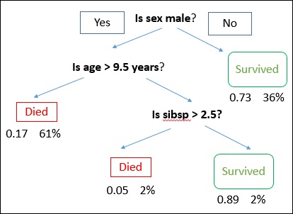
A decision tree is drawn with its root at the top and branches at the bottom. In the image, the bold text represents a condition/internal node, based on which the tree splits into branches/ edges. The branch end that doesn’t split anymore is the decision/leaf.
Example
Consider an example of using titanic data set for predicting whether a passenger will survive or not. The model below uses 3 features/attributes/columns from the data set, namely sex, age and sibsp (no of spouse/children). In this case, whether the passenger died or survived, is represented as red and green text respectively.
In some examples, we see that the population is classified into different groups based on multiple attributes to identify ‘if they do something or not’. To split the population into different heterogeneous groups, it uses various techniques like Gini, Information Gain, Chi-square, entropy etc.
The best way to understand how decision tree works, is to play Jezzball – a classic game from Microsoft. Essentially, in this game, you have a room with moving walls and you need to create walls such that maximum area gets cleared off without the balls.
So, every time you split the room with a wall, you are trying to create 2 different populations with in the same room. Decision trees work in very similar fashion by dividing a population in as different groups as possible.
Observe the code and its output given below −
#Starting implementation
import pandas as pd
import matplotlib.pyplot as plt
import numpy as np
import seaborn as sns
%matplotlib inline
from sklearn import tree
df = pd.read_csv("iris_df.csv")
df.columns = ["X1", "X2", "X3","X4", "Y"]
df.head()

#implementation
from sklearn.cross_validation import train_test_split
decision = tree.DecisionTreeClassifier(criterion="gini")
X = df.values[:, 0:4]
Y = df.values[:, 4]
trainX, testX, trainY, testY = train_test_split( X, Y, test_size = 0.3)
decision.fit(trainX, trainY)
print("Accuracy: \n", decision.score(testX, testY))

#Visualisation
from sklearn.externals.six import StringIO
from IPython.display import Image
import pydotplus as pydot
dot_data = StringIO()
tree.export_graphviz(decision, out_file=dot_data)
graph = pydot.graph_from_dot_data(dot_data.getvalue())
Image(graph.create_png())
Output
Accuracy:
0.955555555556
Example
Here we are using the banknote authentication dataset to know the accuracy.
# Using the Bank Note dataset
from random import seed
from random import randrange
from csv import reader

# Loading a CSV file
filename ='data_banknote_authentication.csv'
def load_csv(filename):
   file = open(filename, "rb")
   lines = reader(file)
   dataset = list(lines)
   return dataset

# Convert string column to float
def str_column_to_float(dataset, column):
   for row in dataset:
      row[column] = float(row[column].strip())

# Split a dataset into k folds
def cross_validation_split(dataset, n_folds):
   dataset_split = list()
   dataset_copy = list(dataset)
   fold_size = int(len(dataset) / n_folds)
   for i in range(n_folds):
      fold = list()
      while len(fold) < fold_size:
         index = randrange(len(dataset_copy))
         fold.append(dataset_copy.pop(index))
      dataset_split.append(fold)
   return dataset_split

# Calculating accuracy percentage
def accuracy_metric(actual, predicted):
correct = 0
for i in range(len(actual)):
if actual[i] == predicted[i]:
correct += 1
return correct / float(len(actual)) * 100.0

# Evaluating an algorithm using a cross validation split
def evaluate_algorithm(dataset, algorithm, n_folds, *args):
   folds = cross_validation_split(dataset, n_folds)
   scores = list()
   for fold in folds:
      train_set = list(folds)
      train_set.remove(fold)
      train_set = sum(train_set, [])
      test_set = list()
      for row in fold:
         row_copy = list(row)
         test_set.append(row_copy)
         row_copy[-1] = None
      predicted = algorithm(train_set, test_set, *args)
      actual = [row[-1] for row in fold]
      accuracy = accuracy_metric(actual, predicted)
      scores.append(accuracy)
   return scores

# Splitting a dataset based on an attribute and an attribute value
def test_split(index, value, dataset):
   left, right = list(), list()
   for row in dataset:
      if row[index] < value:
         left.append(row)
      else:
         right.append(row)
   return left, right

# Calculating the Gini index for a split dataset
def gini_index(groups, classes):
   # count all samples at split point
   n_instances = float(sum([len(group) for group in groups]))
   # sum weighted Gini index for each group
   gini = 0.0
   for group in groups:
      size = float(len(group))
      # avoid divide by zero
      if size == 0:
         continue
      score = 0.0
      # score the group based on the score for each class
      for class_val in classes:
         p = [row[-1] for row in group].count(class_val) / size
      score += p * p
      # weight the group score by its relative size
      gini += (1.0 - score) * (size / n_instances)
return gini

# Selecting the best split point for a dataset
def get_split(dataset):
   class_values = list(set(row[-1] for row in dataset))
   b_index, b_value, b_score, b_groups = 999, 999, 999, None
   for index in range(len(dataset[0])-1):
      for row in dataset:
         groups = test_split(index, row[index], dataset)
         gini = gini_index(groups, class_values)
         if gini < b_score:
            b_index, b_value, b_score, b_groups = index,
row[index], gini, groups
   return {'index':b_index, 'value':b_value, 'groups':b_groups}

# Creating a terminal node value
def to_terminal(group):
outcomes = [row[-1] for row in group]
return max(set(outcomes), key=outcomes.count)

# Creating child splits for a node or make terminal
def split(node, max_depth, min_size, depth):
   left, right = node['groups']
   del(node['groups'])

   # check for a no split
   if not left or not right:
      node['left'] = node['right'] = to_terminal(left + right)
      return

   # check for max depth
   if depth >= max_depth:
      node['left'], node['right'] = to_terminal(left), to_terminal(right)
      return

   # process left child
   if len(left) <= min_size:
      node['left'] = to_terminal(left)
   else:
      node['left'] = get_split(left)
      split(node['left'], max_depth, min_size, depth+1)
   # process right child
   if len(right) <= min_size:
      node['right'] = to_terminal(right)
   else:
      node['right'] = get_split(right)
      split(node['right'], max_depth, min_size, depth+1)

# Building a decision tree
def build_tree(train, max_depth, min_size):
   root = get_split(train)
   split(root, max_depth, min_size, 1)
   return root

# Making a prediction with a decision tree
   def predict(node, row):
   if row[node['index']] < node['value']:
      if isinstance(node['left'], dict):
         return predict(node['left'], row)
      else:
         return node['left']
   else:
      if isinstance(node['right'], dict):
         return predict(node['right'], row)
      else:
         return node['right']

# Classification and Regression Tree Algorithm
def decision_tree(train, test, max_depth, min_size):
   tree = build_tree(train, max_depth, min_size)
   predictions = list()
   for row in test:
      prediction = predict(tree, row)
      predictions.append(prediction)
   return(predictions)

# Testing the Bank Note dataset
seed(1)
# load and prepare data
filename = 'data_banknote_authentication.csv'
dataset = load_csv(filename)

# convert string attributes to integers
for i in range(len(dataset[0])):
   str_column_to_float(dataset, i)

# evaluate algorithm
n_folds = 5
max_depth = 5
min_size = 10
scores = evaluate_algorithm(dataset, decision_tree, n_folds, max_depth, min_size)
print('Scores: %s' % scores)
print('Mean Accuracy: %.3f%%' % (sum(scores)/float(len(scores))))
When you execute the code given above, you can observe the output as follows −
Scores: [95.62043795620438, 97.8102189781022, 97.8102189781022,
94.52554744525547, 98.90510948905109]

Mean Accuracy: 96.934%
Support Vector Machines (SVM)
Support vector machines, also known as SVM, are well-known supervised classification algorithms that separate different categories of data.
These vectors are classified by optimizing the line so that the closest point in each of the groups will be the farthest away from each other.
This vector is by default linear and is also often visualized as being linear. However, the vector can also take a nonlinear form as well if the kernel type is changed from the default type of ‘gaussian’ or linear.
It is a classification method, where we plot each data item as a point in n-dimensional space (where n is number of features) with the value of each feature being the value of a particular coordinate.
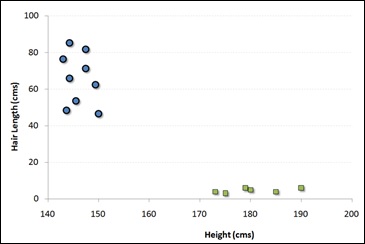
For example, if we have only two features like Height and Hair length of an individual, we should first plot these two variables in two dimensional space where each point has two co-ordinates known as Support Vectors. Observe the following diagram for better understanding −
Now, find some line that splits the data between the two differently classified groups of data. This will be the line such that the distances from the closest point in each of the two groups will be farthest away.
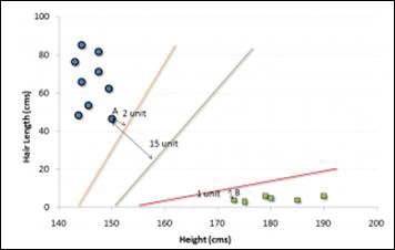
In the example shown above, the line which splits the data into two differently classified groups is the black line, since the two closest points are the farthest apart from the line. This line is our classifier. Then, depending on where the testing data lands on either side of the line, we can classify the new data.
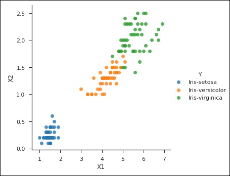
from sklearn import svm
df = pd.read_csv('iris_df.csv')
df.columns = ['X4', 'X3', 'X1', 'X2', 'Y']
df = df.drop(['X4', 'X3'], 1)
df.head()
from sklearn.cross_validation import train_test_split
support = svm.SVC()
X = df.values[:, 0:2]
Y = df.values[:, 2]
trainX, testX, trainY, testY = train_test_split( X, Y, test_size = 0.3)
sns.set_context('notebook', font_scale=1.1)
sns.set_style('ticks')
sns.lmplot('X1','X2', scatter=True, fit_reg=False, data=df, hue='Y')
plt.ylabel('X2')
plt.xlabel('X1')
You can notice the following output and plot when you run the code shown above −
Text(0.5,27.256,'X1')
Naïve Bayes Algorithm
It is a classification technique based on Bayes’ theorem with an assumption that predictor variables are independent. In simple words, a Naive Bayes classifier assumes that the presence of a particular feature in a class is not related to the presence of any other feature.
For example, a fruit may be considered to be an orange if it is orange in color, round, and about 3 inches in diameter. Even if these features are dependent on each other or upon the existence of the other features, a naive Bayes classifier would consider all of these characteristics to independently contribute to the probability that this fruit is an orange.
Naive Bayesian model is easy to make and particularly useful for very large data sets. Apart from being simple, Naive Bayes is known to outperform even highly advanced classification methods.
Bayes theorem provides a way of calculating posterior probability P(c|x) from P(c), P(x) and P(x|c). Observe the equation provided here: P(c/x) = P(x/c)P(c)/P(x)
where,
P(c|x) is the posterior probability of class (target) given predictor (attribute).
P(c) is the prior probability of class.
P(x|c) is the likelihood which is the probability of predictor given class.
P(x) is the prior probability of predictor.
Consider the example given below for a better understanding −
Assume a training data set of Weather and corresponding target variable Play. Now, we need to classify whether players will play or not based on weather condition. For this you will have to take the steps shown below −
Step 1 − Convert the data set to frequency table.
Step 2 − Create Likelihood table by finding the probabilities like Overcast probability = 0.29 and probability of playing is 0.64.
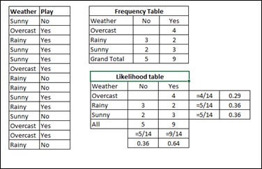
Step 3 − Now, use Naive Bayesian equation to calculate the posterior probability for each class. The class with the highest posterior probability is the outcome of prediction.
Problem − Players will play if weather is sunny, is this statement correct?
Solution − We can solve it using the method discussed above, so P(Yes | Sunny) = P( Sunny | Yes) * P(Yes) / P (Sunny)
Here we have, P (Sunny |Yes) = 3/9 = 0.33, P(Sunny) = 5/14 = 0.36, P(Yes) = 9/14 = 0.64
Now, P (Yes | Sunny) = 0.33 * 0.64 / 0.36 = 0.60, which has a higher probability.
Naive Bayes uses a similar method to predict the probability of different classes based on various attributes. This algorithm is mostly used in text classification and with problems having multiple classes.
The following code shows an example of Naive Bayes implementation −
import csv
import random
import math

def loadCsv(filename):
   lines = csv.reader(open(filename, "rb"))
   dataset = list(lines)
   for i in range(len(dataset)):
      dataset[i] = [float(x) for x in dataset[i]]
   return dataset

def splitDataset(dataset, splitRatio):
   trainSize = int(len(dataset) * splitRatio)
   trainSet = []
   copy = list(dataset)
   while len(trainSet) < trainSize:
      index = random.randrange(len(copy))
      trainSet.append(copy.pop(index))
   return [trainSet, copy]

def separateByClass(dataset):
   separated = {}
   for i in range(len(dataset)):
      vector = dataset[i]
      if (vector[-1] not in separated):
         separated[vector[-1]] = []
      separated[vector[-1]].append(vector)
return separated

def mean(numbers):
return sum(numbers)/float(len(numbers))

def stdev(numbers):
   avg = mean(numbers)
   variance = sum([pow(x-avg,2) for x in numbers])/float(len(numbers)-1)
   return math.sqrt(variance)

def summarize(dataset):
   summaries = [(mean(attribute), stdev(attribute)) for attribute in zip(*dataset)]

def summarizeByClass(dataset):
   separated = separateByClass(dataset)
   summaries = {}
   for classValue, instances in separated.iteritems():
      summaries[classValue] = summarize(instances)
   return summaries

def calculateProbability(x, mean, stdev):
   exponent = math.exp(-(math.pow(x-mean,2)/(2*math.pow(stdev,2))))
   return (1 / (math.sqrt(2*math.pi) * stdev)) * exponent

def calculateClassProbabilities(summaries, inputVector):
   probabilities = {}
   for classValue, classSummaries in summaries.iteritems():
      probabilities[classValue] = 1
      for i in range(len(classSummaries)):
      mean, stdev = classSummaries[i]
      x = inputVector[i]
      probabilities[classValue] *= calculateProbability(x, mean,stdev)
   return probabilities

def predict(summaries, inputVector):
   probabilities = calculateClassProbabilities(summaries, inputVector)
   bestLabel, bestProb = None, -1
   for classValue, probability in probabilities.iteritems():
      if bestLabel is None or probability > bestProb:
         bestProb = probability
         bestLabel = classValue
   return bestLabel

def getPredictions(summaries, testSet):
   predictions = []
   for i in range(len(testSet)):
      result = predict(summaries, testSet[i])
      predictions.append(result)
   return predictions

def getAccuracy(testSet, predictions):
   correct = 0
   for i in range(len(testSet)):
      if testSet[i][-1] == predictions[i]:
         correct += 1
   return (correct/float(len(testSet))) * 100.0

def main():
   filename = 'pima-indians-diabetes.data.csv'
   splitRatio = 0.67
   dataset = loadCsv(filename)
   trainingSet, testSet = splitDataset(dataset, splitRatio)
   print('Split {0} rows into train = {1} and test = {2} rows').format(len(dataset), len(trainingSet), len(testSet))
   # prepare model
   summaries = summarizeByClass(trainingSet)
   # test model
   predictions = getPredictions(summaries, testSet)
   accuracy = getAccuracy(testSet, predictions)
   print('Accuracy: {0}%').format(accuracy)
main()
When you run the code given above, you can observe the following output −
Split 1372 rows into train = 919 and test = 453 rows

Accuracy: 83.6644591611%
KNN (K-Nearest Neighbours)
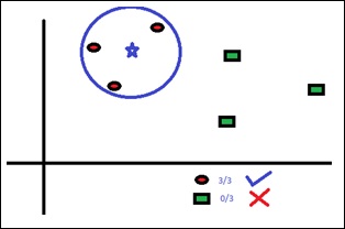
K-Nearest Neighbors, KNN for short, is a supervised learning algorithm specialized in classification. It is a simple algorithm that stores all available cases and classifies new cases by a majority vote of its k neighbors. The case being assigned to the class is the most common among its K nearest neighbors measured by a distance function. These distance functions can be Euclidean, Manhattan, Minkowski and Hamming distance. First three functions are used for continuous function and fourth one (Hamming) for categorical variables. If K = 1, then the case is simply assigned to the class of its nearest neighbor. At times, choosing K turns out to be a challenge while performing KNN modeling.
The algorithm looks at different centroids and compares distance using some sort of function (usually Euclidean), then analyzes those results and assigns each point to the group so that it is optimized to be placed with all the closest points to it.
You can use KNN for both classification and regression problems. However, it is more widely used in classification problems in the industry. KNN can easily be mapped to our real lives.
You will have to note the following points before selecting KNN −
- KNN is computationally expensive.
- Variables should be normalized else higher range variables can bias it.
- Works on pre-processing stage more before going for KNN like outlier, noise removal
Observe the following code for a better understanding of KNN −
#Importing Libraries
from sklearn.neighbors import KNeighborsClassifier
#Assumed you have, X (predictor) and Y (target) for training data set and x_test(predictor) of test_dataset
# Create KNeighbors classifier object model
KNeighborsClassifier(n_neighbors=6) # default value for n_neighbors is 5
# Train the model using the training sets and check score
model.fit(X, y)
#Predict Output
predicted= model.predict(x_test)
from sklearn.neighbors import KNeighborsClassifier
df = pd.read_csv('iris_df.csv')
df.columns = ['X1', 'X2', 'X3', 'X4', 'Y']
df = df.drop(['X4', 'X3'], 1)
df.head()
sns.set_context('notebook', font_scale=1.1)
sns.set_style('ticks')
sns.lmplot('X1','X2', scatter=True, fit_reg=False, data=df, hue='Y')
plt.ylabel('X2')
plt.xlabel('X1')
from sklearn.cross_validation import train_test_split
neighbors = KNeighborsClassifier(n_neighbors=5)
X = df.values[:, 0:2]
Y = df.values[:, 2]
trainX, testX, trainY, testY = train_test_split( X, Y, test_size = 0.3)
neighbors.fit(trainX, trainY)
print('Accuracy: \n', neighbors.score(testX, testY))
pred = neighbors.predict(testX)
The code given above will produce the following output −
('Accuracy: \n', 0.75555555555555554)
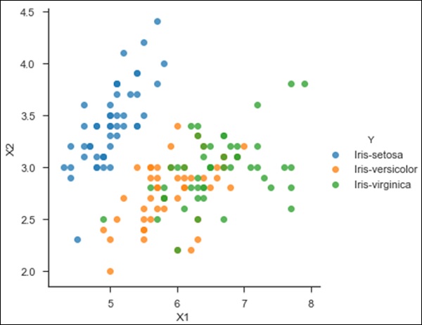
K-Means
It is a type of unsupervised algorithm which deals with the clustering problems. Its procedure follows a simple and easy way to classify a given data set through a certain number of clusters (assume k clusters). Data points inside a cluster are homogeneous and are heterogeneous to peer groups.
How K-means Forms Cluster
K-means forms cluster in the steps given below −
- K-means picks k number of points for each cluster known as centroids.
- Each data point forms a cluster with the closest centroids, that is k clusters.
- Finds the centroid of each cluster based on existing cluster members. Here we have new centroids.
As we have new centroids, repeat step 2 and 3. Find the closest distance for each data point from new centroids and get associated with new k-clusters. Repeat this process until convergence occurs, that is till centroids do not change.
Determination of Value of K
In K-means, we have clusters and each cluster has its own centroid. Sum of square of difference between centroid and the data points within a cluster constitutes the sum of square value for that cluster. Also, when the sum of square values for all the clusters are added, it becomes total within sum of square value for the cluster solution.
We know that as the number of cluster increases, this value keeps on decreasing but if you plot the result you may see that the sum of squared distance decreases sharply up to some value of k, and then much more slowly after that. Here, we can find the optimum number of cluster.
Observe the following code −
import numpy as np
import matplotlib.pyplot as plt
from matplotlib import style
style.use("ggplot")
from sklearn.cluster import KMeans
x = [1, 5, 1.5, 8, 1, 9]
y = [2, 8, 1.8, 8, 0.6, 11]

plt.scatter(x,y)
plt.show()
X = np.array([ [1, 2],
               [5, 8],
               [1.5, 1.8],
               [8, 8],
               [1, 0.6],
               [9, 11]])
kmeans = KMeans(n_clusters=2)
kmeans.fit(X)
centroids = kmeans.cluster_centers_
labels = kmeans.labels_
print(centroids)
print(labels)
colors = ["g.","r.","c.","y."]

for i in range(len(X)):
   print("coordinate:",X[i], "label:", labels[i])
   plt.plot(X[i][0], X[i][1], colors[labels[i]], markersize = 10)
plt.scatter(centroids[:, 0],centroids[:, 1], marker = "x", s=150, linewidths = 5, zorder = 10)
plt.show()
When you run the code given above, you can see the following output −
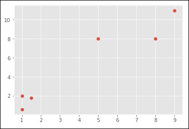
[ [ 1.16666667 1.46666667] [ 7.33333333 9. ] ]
[0 1 0 1 0 1]
('coordinate:', array([ 1., 2.]), 'label:', 0)
('coordinate:', array([ 5., 8.]), 'label:', 1)
('coordinate:', array([ 1.5, 1.8]), 'label:', 0)
('coordinate:', array([ 8., 8.]), 'label:', 1)
('coordinate:', array([ 1. , 0.6]), 'label:', 0)
('coordinate:', array([ 9., 11.]), 'label:', 1)
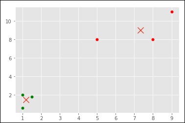
Here is another code for your understanding −
from sklearn.cluster import KMeans
df = pd.read_csv('iris_df.csv')
df.columns = ['X1', 'X2', 'X3', 'X4', 'Y']
df = df.drop(['X4', 'X3'], 1)
df.head()
from sklearn.cross_validation import train_test_split
kmeans = KMeans(n_clusters = 3)
X = df.values[:, 0:2]
kmeans.fit(X)
df['Pred'] = kmeans.predict(X)
df.head()
sns.set_context('notebook', font_scale = 1.1)
sns.set_style('ticks')
sns.lmplot('X1','X2', scatter = True, fit_reg = False, data = df, hue = 'Pred')
Here is the output of the above code −
<seaborn.axisgrid.FacetGrid at 0x107ad6a0>
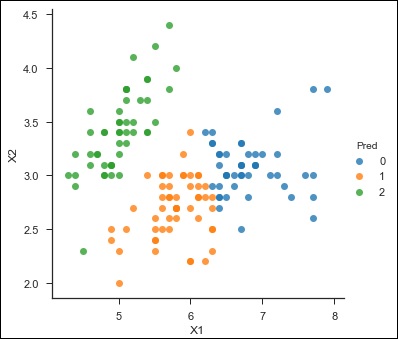
Random Forest
Random Forest is a popular supervised ensemble learning algorithm. ‘Ensemble’ means that it takes a bunch of ‘weak learners’ and has them work together to form one strong predictor. In this case, the weak learners are all randomly implemented decision trees that are brought together to form the strong predictor — a random forest.
Observe the following code −
from sklearn.ensemble import RandomForestClassifier
df = pd.read_csv('iris_df.csv')
df.columns = ['X1', 'X2', 'X3', 'X4', 'Y']
df.head()
from sklearn.cross_validation import train_test_split
forest = RandomForestClassifier()
X = df.values[:, 0:4]
Y = df.values[:, 4]
trainX, testX, trainY, testY = train_test_split( X, Y, test_size = 0.3)
forest.fit(trainX, trainY)
print('Accuracy: \n', forest.score(testX, testY))
pred = forest.predict(testX)
The output for the code given above is −
('Accuracy: \n', 1.0)
The goal of ensemble methods is to combine the predictions of several base estimators built with a given learning algorithm in order to improve generalizability / robustness over a single estimator.
The sklearn.ensemble module includes two averaging algorithms based on randomized decision trees - the RandomForest algorithm and the Extra-Trees method. Both algorithms are perturb-and-combine techniques [B1998] specifically designed for trees. This means a diverse set of classifiers is created by introducing randomness in the classifier construction. The prediction of the ensemble is given as the averaged prediction of the individual classifiers.
Forest classifiers have to be fitted with two arrays - a sparse or dense array X of size [n_samples, n_features] holding the training samples, and an array Y of size [n_samples] holding the target values (class labels) for the training samples, as shown in the code below −
>>> from sklearn.ensemble import RandomForestClassifier
>>> X = [[0, 0], [1, 1]]
>>> Y = [0, 1]
>>> clf = RandomForestClassifier(n_estimators = 10)
>>> clf = clf.fit(X, Y)
Like decision trees, forests of trees also extend to multi-output problems (if Y is an array of size [n_samples, n_outputs]).
In contrast to the original publication [B2001], the scikit-learnimplementation combines classifiers by averaging their probabilistic prediction, instead of letting each classifier vote for a single class.
Random Forest is a trademark term for an ensemble of decision trees. In Random Forest, we have a collection of decision trees, known as “Forest”. To classify a new object based on attributes, each tree gives a classification and we say the tree “votes” for that class. The forest chooses the classification having the most votes (over all the trees in the forest).
Each tree is planted & grown as follows −
- If the number of cases in the training set is N, then sample of N cases is taken at random but with replacement. This sample will be the training set for growing the tree.
- If there are M input variables, a number m<<M is specified such that at each node, m variables are selected at random out of the M and the best split on these m is used to split the node. The value of m is held constant during the forest growing.
- Each tree is grown to the largest extent possible. There is no pruning.
Dimensionality Reduction Algorithm
Dimensionality reduction is yet another common unsupervised learning task. Some problems may contain tens of thousands or even millions of input or explanatory variables, which can be costly to work with and do computations. Moreover, the program's ability to generalize may be diminished if some of the input variables capture noise or are not relevant to the underlying relationship.
Dimensionality reduction is the process of finding the input variables that are responsible for the greatest changes in the output or response variable. Dimensionality reduction is sometimes also used to visualize data. It is easy to visualize a regression problem such as predicting the price of a property from its size, where the size of the property can be plotted along graph's x axis, and the price of the property can be plotted along the y axis. Similarly, it is easy to visualize the property price regression problem when a second explanatory variable is added. The number of rooms in the property could be plotted on the z axis, for instance. A problem with thousands of input variables, however, becomes impossible to visualize.
Dimensionality reduction, reduces a very large set of input of explanatory variables to a smaller set of input variables that retain as much information as possible.
PCA is a dimensionality reduction algorithm that can do useful things for data analysis. Most importantly, it can dramatically reduce the number of computations involved in a model when dealing with hundreds or thousands of different input variables. As it is an unsupervised learning task, the user still has to analyze the results and make sure they are keeping 95% or so of the original dataset’s behavior.
Observe the following code for a better understanding −
from sklearn import decomposition
df = pd.read_csv('iris_df.csv')
df.columns = ['X1', 'X2', 'X3', 'X4', 'Y']
df.head()
from sklearn import decomposition
pca = decomposition.PCA()
fa = decomposition.FactorAnalysis()
X = df.values[:, 0:4]
Y = df.values[:, 4]
train, test = train_test_split(X,test_size = 0.3)
train_reduced = pca.fit_transform(train)
test_reduced = pca.transform(test)
pca.n_components_
You can see the following output for the code given above −
4L
In the last 5 years, there has been an exponential rise in data capturing at every possible level and point. Government Agencies/ Research Organizations/Corporates are not only coming out with new data sources, but also they are capturing very detailed data at several points and stages.
For example, e-commerce companies are capturing more details about customers like their demographics, browsing history, their likes or dislikes, purchase history, feedback and several other details to give them customized attention. The data that is now available may have thousands of features and reducing those features while retaining as much information as possible is a challenge. In such situations, dimensionality reduction helps a lot.
Boosting Algorithms
The term ‘Boosting’ refers to a family of algorithms that converts weak learner to strong learners. Let us understand this definition by solving a problem of spam email identification as shown below −
What procedure should be followed to classify an email as SPAM or not? In initial approach, we would identify ‘spam’ and ‘not spam’ emails using following criteria if −
- Email has only one image file (advertisement image), It’s a SPAM
- Email has only link(s), It’s a SPAM
- Email body consist of sentence like “You won a prize money of $ xxxxxx”, It’s a SPAM
- Email from our official domain “Tutorialspoint.com” , Not a SPAM
- Email from known source, Not a SPAM
Above, we have defined several rules to classify an email into ‘spam’ or ‘not spam’. These rules, however, individually are not strong enough to successfully classify an email into ‘spam’ or ‘not spam’. Therefore, these rules are termed as weak learner.
To convert weak learner to strong learner, we combine the prediction of each weak learner using methods like −
- Using average/weighted average
- Considering prediction that has higher vote
For example, suppose we have defined 7 weak learners. Out of these 7, 5 are voted as ‘SPAM’ and 2 are voted as ‘Not a SPAM’. In this case, by default, we’ll consider an email as SPAM because we have higher (5) vote for ‘SPAM’.
How It Works
Boosting combines weak learner or base learner to form a strong rule. This section will explain you how boosting identifies weak rules.
To find weak rule, we apply base learning (ML) algorithms with a different distribution. Each time base learning algorithm is applied, it generates a new weak prediction rule. This uses iteration processes several times. After many iterations, the boosting algorithm combines these weak rules into a single strong prediction rule.
For choosing the right distribution for each round, follow the given steps −
Step 1 − The base learner takes all the distributions and assigns equal weight to each one.
Step 2 − If there is any prediction error caused by first base learning algorithm, then we pay higher weight to observations having prediction error. Then, we apply the next base learning algorithm.
We iterate Step 2 till the limit of base learning algorithm is attained or higher accuracy is achieved.
Finally, it combines the outputs from weak learner and makes a strong learner which eventually improves the prediction power of the model. Boosting lays more focus on examples which are wrongly classified or have higher errors by due to weak rules.
Types of Boosting Algorithms
There are several types of engine used for boosting algorithms - decision stump, margin-maximizing classification algorithm and so on. Different boosting algorithms are listed here −
- AdaBoost (Adaptive Boosting)
- Gradient Tree Boosting
- XGBoost
This section focuses on AdaBoost and Gradient Boosting followed by their respective Boosting Algorithms.
AdaBoost
Observe the following figure that explains Ada-boost algorithm.
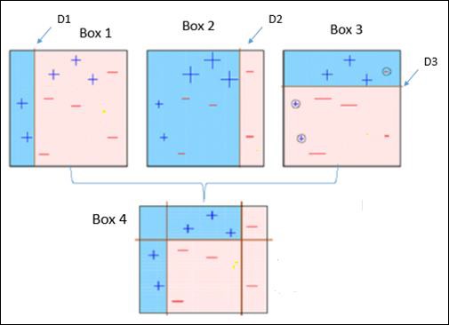
It is explained below −
Box 1 − You can see that we have assigned equal weights to each data point and applied a decision stump to classify them as + (plus) or – (minus). The decision stump (D1) has created a vertical line at left side to classify the data points. This vertical line has incorrectly predicted three + (plus) as – (minus). So, we’ll assign higher weights to these three + (plus) and apply another decision stump.
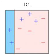
Box 2 − Here, it can see that the size of three (wrongly predicted) + (plus) data points is bigger as compared to rest of the data points. In this case, the second decision stump (D2) will try to predict them correctly. Now, a vertical line (D2) at right side of this box has classified three wrongly classified + (plus) correctly. But again, it has made mis-classification errors. This time with three -(minus) data points. Again, we will assign higher weights to the three – (minus) data points and apply another decision stump.
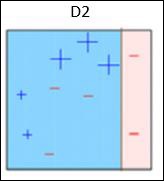
Box 3 − Here, three – (minus) data points are given higher weights. A decision stump (D3) is applied to predict these wrongly classified observations correctly. This time a horizontal line is generated to classify + (plus) and – (minus) data points based on higher weight of wrongly classified observations.
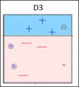
Box 4 − Here, we have joined D1, D2 and D3 to form a strong prediction having complex rule as compared to individual weak learners. It can be seen that this algorithm has classified these observations quite well as compared to any of individual weak learner.
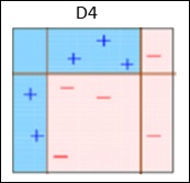
AdaBoost or Adaptive Boosting − It works on similar method as discussed above. It fits a sequence of weak learners on different weighted training data. It starts by predicting original data set and gives equal weight to each observation. If prediction is incorrect using the first learner, then it gives higher weight to observations which have been predicted incorrectly. Being an iterative process, it continues to add learner(s) until a limit is reached in the number of models or accuracy.
Mostly, we use decision stamps with AdaBoost. But, we can use any machine learning algorithms as base learner if it accepts weight on training data set. We can use AdaBoost algorithms for both classification and regression problems.
You can use the following Python code for this purpose −
#for classification
from sklearn.ensemble import AdaBoostClassifier
#for regression
from sklearn.ensemble import AdaBoostRegressor
from sklearn.tree import DecisionTreeClassifier
dt = DecisionTreeClassifier()
clf = AdaBoostClassifier(n_estimators=100, base_estimator=dt,learning_rate=1)
#Here we have used decision tree as a base estimator; Any ML learner can be used as base #estimator if it accepts sample weight
clf.fit(x_train,y_train)
Parameters for Tuning
The parameters can be tuned to optimize the performance of algorithms, The key parameters for tuning are −
n_estimators − These control the number of weak learners.
learning_rate − This controls the contribution of weak learners in the final combination. There is a trade-off between learning_rate and n_estimators.
base_estimators − These help to specify different ML algorithm.
The parameters of base learners can also be tuned to optimize its performance.
Gradient Boosting
In gradient boosting, many models are trained sequentially. Each new model gradually minimizes the loss function (y = ax + b + e, where ‘e’ is the error term) of the whole system using Gradient Descent method. The learning method consecutively fits new models to give a more accurate estimate of the response variable.
The main idea behind this algorithm is to construct new base learners which can be optimally correlated with negative gradient of the loss function, relevant to the whole ensemble.
In Python Sklearn library, we use Gradient Tree Boosting or GBRT which is a generalization of boosting to arbitrary differentiable loss functions. It can be utilized for both regression and classification problems.
You can use the following code for this purpose −
#for classification
from sklearn.ensemble import GradientBoostingClassifier
#for regression
from sklearn.ensemble import GradientBoostingRegressor
clf = GradientBoostingClassifier(n_estimators = 100, learning_rate = 1.0, max_depth = 1)
clf.fit(X_train, y_train)
Here are the terms used in the above code −
n_estimators − These control the number of weak learners.
learning_rate − This controls the contribution of weak learners in the final combination. There is a trade-off between learning_rate and n_estimators.
max_depth − This is the maximum depth of the individual regression estimators which limits the number of nodes in the tree. This parameter is tuned for best performance and the best value depends on the interaction of the input variables.
The loss function can be tuned for better performance.
Machine Learning with Python - Applications
Artificial Intelligence (AI) and Machine Learning are everywhere. Chances are that you are using them and not even aware about that. In Machine Learning (ML), computers, software, and devices perform via cognition similar to human brain.
Typical successful applications of machine learning include programs that decode handwritten text, face recognition, voice recognition, speech recognition, pattern recognition, spam detection programs, weather forecasting, stock market analysis and predictions, and so on. This chapter discusses these applications in detail.
Virtual Personal Assistants
Siri, Google Now, Alexa are some of the common examples of virtual personal assistants. These applications assist in finding information, when asked over voice. All that is needed is activating them and asking questions like for example “What are my appointments for today?”, “What are the flights from Delhi to New York”. For answering such queries, the application looks out for the information, recalls your previous queries, and accesses other resources to collect relevant information. You can even tell these assistants to do certain tasks like “Set an alarm for 5.30 AM next morning”, “Remind me to visit Passport office tomorrow at 10.30 am”.
Traffic Congestion Analysis and Predictions
GPS navigation services monitor the user’s location and velocities and use them to build a map of current traffic. This helps in preventing the traffic congestions. Machine learning in such scenarios helps to estimate the regions where congestion can be found based on previous records.
Automated Video Surveillance
Video surveillance systems nowadays are powered by AI and machine learning is the technology behind this that makes it possible to detect and prevent crimes before they occur. They track odd and suspicious behavior of people and sends alerts to human attendants, who can ultimately help accidents and crimes.
Social Media
Facebook continuously monitors the friends that you connect with, your interests, workplace, or a group that you share with someone etc. Based on continuous learning, a list of Facebook users is given as friend suggestions.
Face Recognition
You upload a picture of you with a friend and Facebook instantly recognizes that friend. Machine learning works at the core of Computer Vision, which is a technique to extract useful information from images and videos. Pinterest uses computer vision to identify objects or pins in the images and recommend similar pins to its users.
Email Spam and Malware Filtering
Machine learning is being extensively used in spam detection and malware filtering and the databases of such spams and malwares keep on getting updated so these are handled efficiently.
Online Customer Support
In several websites nowadays, there is an option to chat with customer support representative while users are navigating the site. In most of the cases, instead of a real executive, you talk to a chatbot. These bots extract information from the website and provide it to the customers to assist them. Over a period of time, the chatbots learn to understand the user queries better and serve them with better answers, and this is made possible by machine learning algorithms.
Refinement of Search Engine Results
Google and similar search engines are using machine learning to improve the search results for their users. Every time a search is executed, the algorithms at the backend keep a watch at how the users respond to the results. Depending on the user responses, the algorithms working at the backend improve the search results.
Product Recommendations
If a user purchases or searches for a product online, he/she keeps on receiving emails for shopping suggestions and ads about that product. Based on previous user behavior, on a website/app, past purchases, items liked or added to cart, brand preferences etc., the product recommendations are sent to the user.
Detection of Online frauds
Machine learning is used to track monetary frauds online. For example - Paypal is using ML to prevent money laundering. The company is using a set of tools that helps them compare millions of transactions and make a distinction between legal or illegal transactions taking place between the buyers and sellers.
Great Article
ReplyDeleteMachine Learning Projects for Students
Final Year Project Centers in Chennai
Thanks for the blog article.Much thanks again. Fantastic.
ReplyDeleteData Science Training
Learn Data Science Online Course